OPTIMIZATION PROBLEM OF EXCESS-OF-LOSS REINSURANCE AND INVESTMENT WITH DELAY AND MISPRICING UNDER THE JUMP-DIFFUSION MODEL

HUANG Qing, MA Shi-xia, GONG Xiao-qin

(School of Science, Hebei University of Technology, Tianjin 300401, China)

Abstract: In this paper, we study an optimization problem of excess-of-loss reinsurance and investment with delay and mispricing under the Jump-diffusion model.Using the stochastic control theory, the equilibrium reinsurance-investment strategy and the corresponding equilibrium value function are derived by solving an extended HJB system.Finally, some special cases of our model and results are presented, and some numerical examples for our results are provided.

Keywords: excess-of-loss reinsurance; Lvy insurance model; mispricing; stochastic differential delay equation; jump-diffusion model

1 Introduction

An insurer can control risks through a number of measures, such as investment and reinsurance.In recent years, the problem of the optimal investment and reinsurance has been widely investigated, which was considered in the literature [1–3]and so on.

With the deepening of research in the insurance field, some scholars point out that the risky asset’s price process is represented by a jump-diffusion model,which is more consistent with the stock market.Ignoring jump risks on risky asset’s price process have an important impact on the optimal problem (see [4,5]).A et al.[6]showed that the development of realworld systems depends not only on their current state but also on their previous history.If we believe that financial market exists bounded memory or the performance-related capital inflow(outflow),then the wealth process with delay must be considered(see[7]).In addition,due to the existence of frictions in markets which are not absolutely mature, insurers can make a profit by mispricing, that is, by exploiting the price difference between a pair of stocks, we can refer to [8,9].

On the basis of previous literature,we establish a class of generalized optimal investment and reinsurance risk model, we consider the optimization problem of excess-of-loss reinsurance and investment with delay and mispricing under the Jump-diffusion model, and the purpose is to obtain the equilibrium reinsurance-investment strategy and the corresponding equilibrium value function.In which we introduce the performance-related capital inflow(outflow)and the price processes of stocks are described by jump-diffusion models with mispricing.Moreover, referring to Li et al.[10], the claim process is described by a spectrally negative Lvy process.

The remainder of this paper is organized as follows.Section 2 gives the model framework.Section 3 derives the explicit expressions of the equilibrium reinsurance-investment strategy and the corresponding equilibrium value function, and provides two special cases of our model.Section 4 provides some numerical examples for sensitivity analysis.

2 The Model

Let(Ω,F,{Ft}t∈[0,T],P)be a complete probability space that fulfills the usual condition,where [0,T]is a fixed and finite time horizon; Ftis the information of the market available up to time t and P is a reference measure.

Following the idea suggested by Li et al.[10], without reinsurance and investment, the insurer’s surplus process modeled by a spectrally negative Lévy process defined on this probability space with dynamics

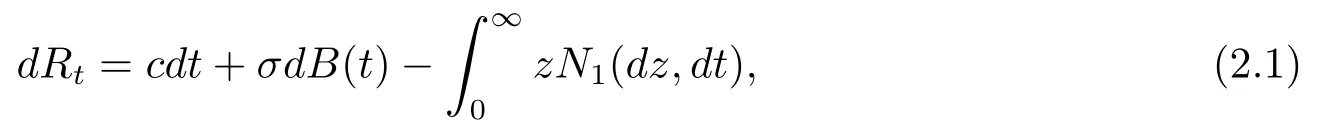
where

(i) N1(dz,dt)is a Poisson random measure representing the number of insurance claims of size (z,z+dz) within the time period (t,t+dt).

(ii) c is the premium rate,according to the expected value principle,where θ >0 is the safety loading of the insurer,σ >0 is the volatility rate,B(t)is a standard Brownian motion.

In theory,we should first suppose that the reinsurance strategy relies on surplus.But in the following Theorem 3.2, we find that the equilibrium reinsurance strategy is independent of the surplus.Thus, for simplicity, we omits possible dependency on the surplus.So the surplus process can be described as

We assume that the insurer is allowed to invest in a financial market composing of one risk-free asset, a market index and a pair of stocks with mispricing (see Gu et al.[8]).The risk-free asset’s price process S0(t) is described by

where r > 0 represents the risk-free interest rate.The price process of the market index Pm(t) follows as

where the market risk premium µmand the market volatility σmare positive constants,and {Zm(t)} is a standard Brownian motion.The price processes of the pair of stocks are described by

(i) µ, σ1, k1and k2are positive constants, σ1dZi(t) describes the risk of stock i in the financial market, i=1,2.

(ii) {N2(t)}t∈[0,T]is homogeneous Poisson process with intensity β1, which represents the number of the price jumps that occurred the first or second stock during time interval[0,T].

(iii) Y1iis the ith jump amplitude of the stock price, and Y1i, i = 1,2,3,··· are i.i.d.random variables.We assume their distribution is G(y1), and they have finite firstorder moment µY1and second-order moment

(iv) Suppose that {Z1(t)}, {Z2(t)}, {Zm(t)}, {B(t)}, N1(dz,dt), andare independent and P(Y1i≥ −1) = 1, i = 1,2,3,··· to guarantee that these two stocks’s prices have always been positive.

(v) The term kjX(t)dt shows the effect of mispricing on the jth stock’s price, j =1,2.

X(t) is the pricing error or mispricing between two stocks, and is defined as

Based on eqs.(2.5) and (2.6), using standard I’s calculus, we find that the dynamics of the mispricing X(t) satisfy the following equation

In addition, we also consider that there exists capital inflow into or outflow from the insurer’s current wealth.We can refer to A et al.[6].Denote the average and pointwise performance of the wealth in the past horizon [t −h,t]by(t) and M(t), respectively, i.e.,

where δ ≥ 0 is an average parameter and h > 0 is the delay parameter.Let Y(t) =thenLet the function g(t,W(t)−represent the capital inflow (outflow) amount which is related to the past performance of the wealth. W(t)−(t) accounts for the average performance of the wealth between t −h and t, and W(t)−M(t) implies the absolute performance of the wealth in the time horizon[t −h,t].

This capital inflow (outflow) may occur in a variety of situations, as described in A et al.[6].We assume that the amount of the capital inflow (outflow) is proportional to the past performance of the insurer’s wealth, i.e.,

where b and c are nonnegative constants.

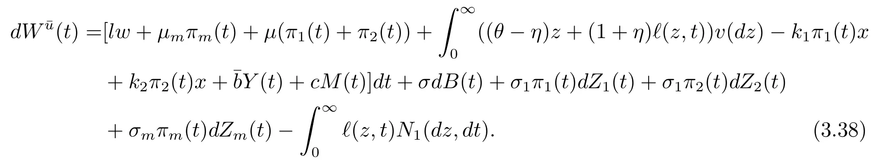
Thus, the insurer’s wealth process {Wu(t),t ∈ [0,T]} is described by

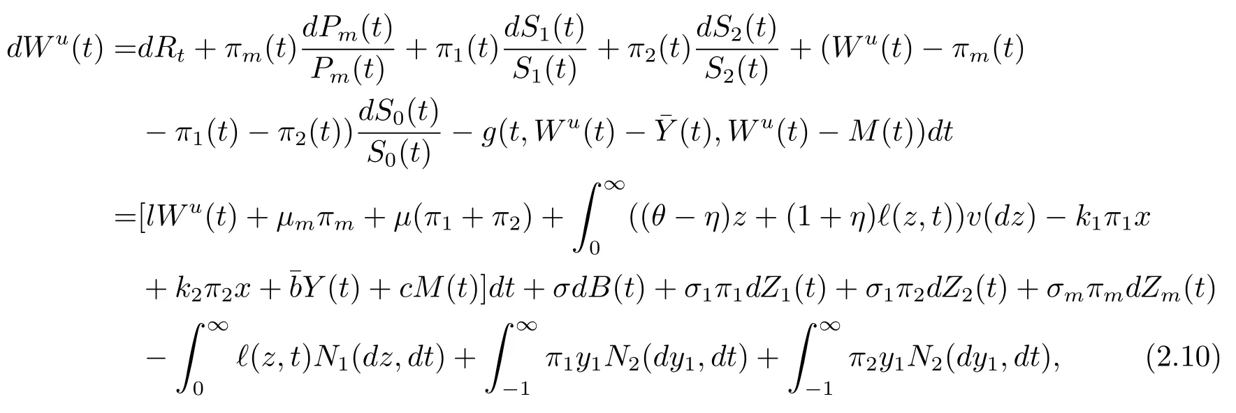
Definition 2.1(Admissible Strategy)A strategy u={ (Zt,t),πm(t),π1(t),π2(t)}t∈[0.T]is admissible if

But fortunately it was almost evening, when the seven dwarfs came home. When they saw Snow-white lying as if dead upon the ground they at once suspected the step-mother, and they looked and found the poisoned comb. Scarcely had they taken it out when Snow-white came to herself, and told them what had happened. Then they warned her once more to be upon her guard and to open the door to no one.

(i) for all t ∈ [0,T], Zt≥ 0, 0 ≤ (Zt,t) ≤ Zt;

(ii)u is predictable w.r.t.{Ft}t∈[0,T],and

(iii) ∀(t,w,x,y) ∈ [0,T]× R × R × [−1,∞), Eq.(2.10) has a pathwise unique solution{Wu(t)}t∈[0.T]with W(t)=w, X(t)=x, Y(t)=y.

Let Π denote the set of all admissible strategies.In this paper, our main purpose is to research the reinsurance and investment problem for an insurer under mean-variance criterion, i.e., wishes to maximize Ju(t,w,x,y), in which Juis given by

where γ > 0 represents a constant absolute risk aversion coefficient.We know that meanvariance criterion has the issue of time-inconsistency.But in many situations,time-consistency of strategies is a basic requirement for rational investors.So, we tackle the problem from a non-cooperative game point of view by defining an equilibrium strategy and its corresponding equilibrium value function (see [11]).

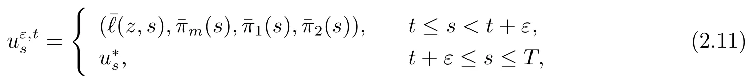
Definition 2.2For an admissible strategyfor ε>0 with any fixed chosen initial state (t,w,x,y)∈ [0,T]×R×R×[−1,∞), define the strategy uε,tby

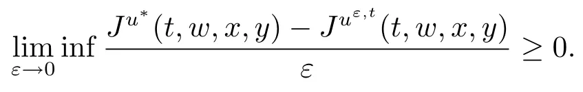
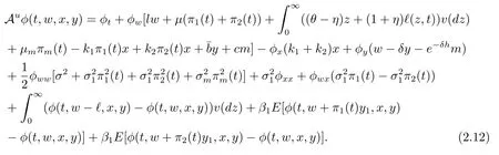
Then u∗is an equilibrium strategy and Ju∗(t,w,x,y)is the corresponding equilibrium value function.For ∀(t,w,x,y) ∈ [0,T]× R × R × [−1,∞), ∀φ(t,w,x,y) ∈ C1,2,2,1([0,T]× R ×R × [−1,∞)), we define a variational operator Auas follows

3 Optimization Problem and the Equilibrium Optimal Strategy

In this section, we consider the optimization problem and seek the optimal strategy,and then analyze two special cases.We first provide a verification theorem whose proof is similar to Theorem 1 of Kryger and Steffensen [12].We omit it here.

then Ju∗(t,w,x,y) = V(t,w,x,y), E[Wu∗(T)]= g(t,w,x,y) and u∗is the equilibrium reinsurance-investment strategy.

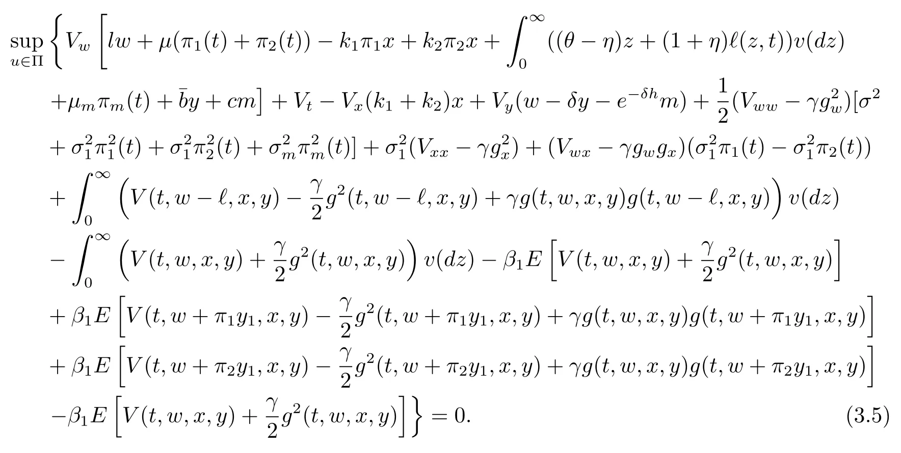
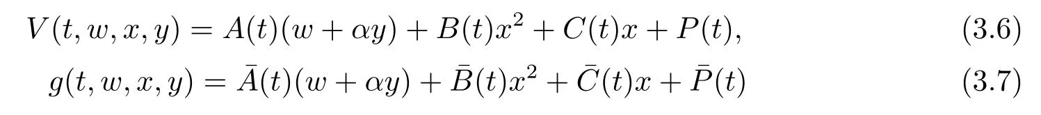
To solve eqs.(3.3) and (3.5), we try to conjecture the solutions in the following forms

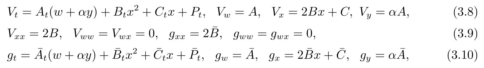
Plugging the above derivatives into (3.5) and simplifying yields

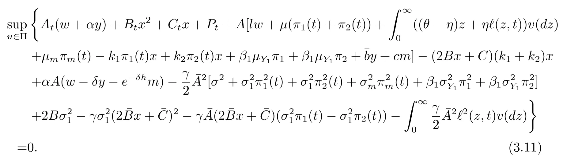
Consider the terms involving in (3.11), that is,

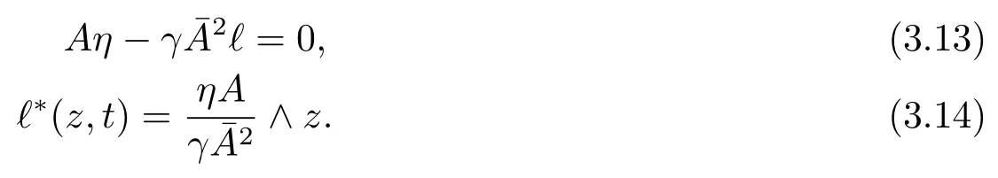
According to Li et al.[10], if we maximize the integrand in the integral in (3.12) zby-z for a given t ∈ [0,T], then we will maximize the integral itself.With respect tothe graph ofis a concave parabola that increases through the origin(0,f(0))=(0,0); by the first-order condition w.r.t.we have

By the first-order condition w.r.t. πm(t), π1(t) and π2(t), we have

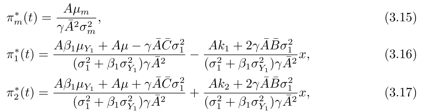
we find that the amounts invested in the two stocks,are functions of x.Plugging eqs.(3.14)–(3.17) into eq.(3.11) and eq.(3.3), we have

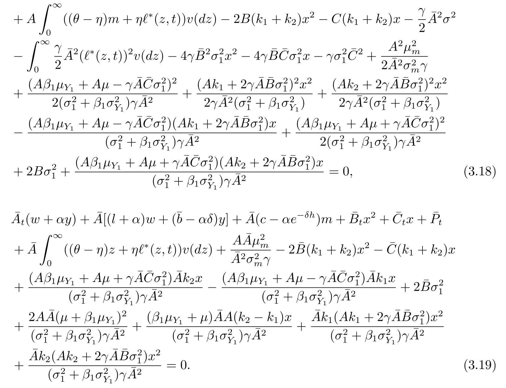
To make the problem solvable, we assume the following conditions on parameters

So, we have A(c −αe−δh)m=0.In order to obtain the expressions oflet At, A,satisfy the following differential equations

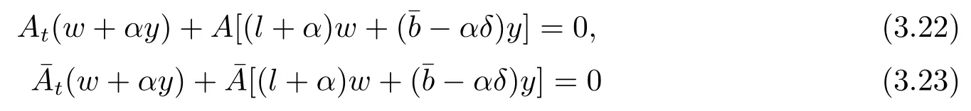
with boundary condition A(T) == 1.Based on condition (3.21), we have−αδ =(l+ α)α.So we have

By separating the variables with and without x, x2, we can derive the following equations

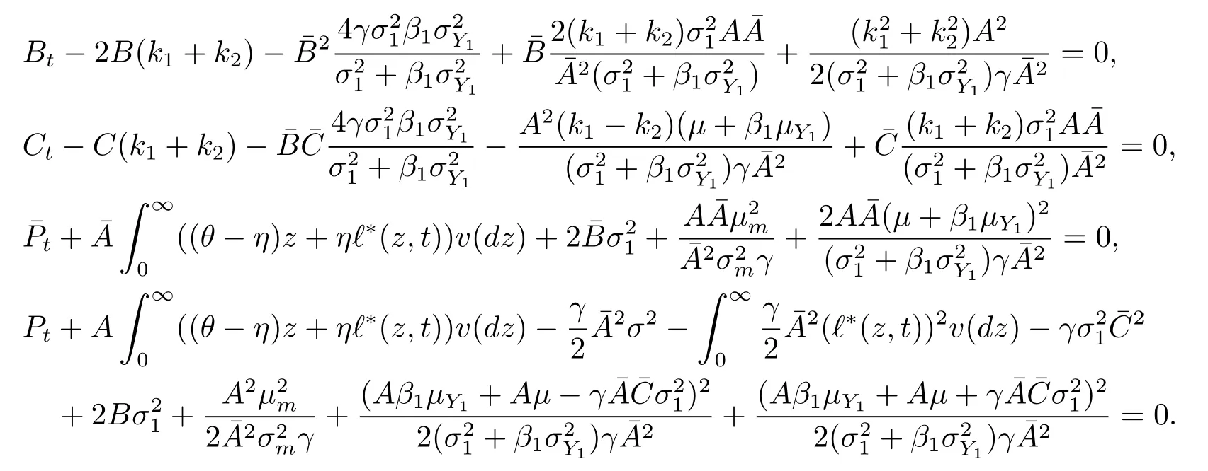
where

Theorem 3.2According to the wealth process (2.10) and the reinsurance-investment problem, the equilibrium value function is

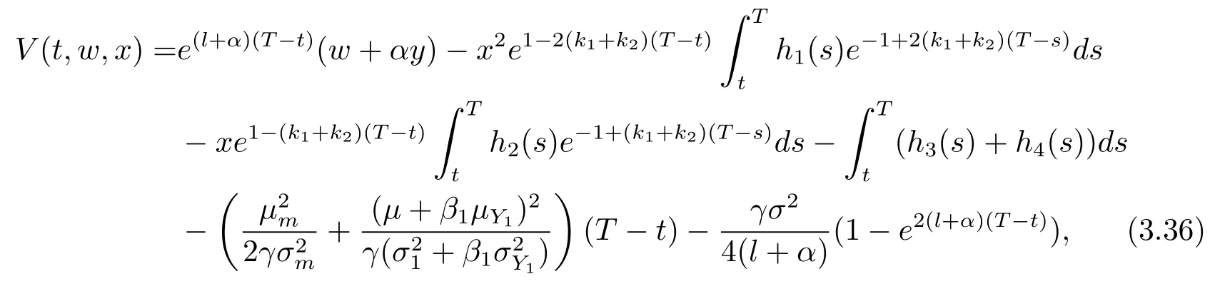
where h1(s), h2(s), h3(s) and h4(s) are given by (3.30)–(3.33).The corresponding equilibrium strategy is given by

In the following sections, we analyze two special cases of our model, i.e., without jump and without mispricing, and give the corresponding equilibrium strategies and equilibrium value functions.

Corollary 3.1 (Without Jump)We consider the optimal reinsurance-investment problem in which the price processes of these two stocks are represented by diffusion models.If we don’t consider jump risk in our model, under the measure P, the wealth process becomes

The corresponding optimization problem becomes

Then, by some similar calculations, the equilibrium reinsurance-investment strategyt ∈[0.T], is given by

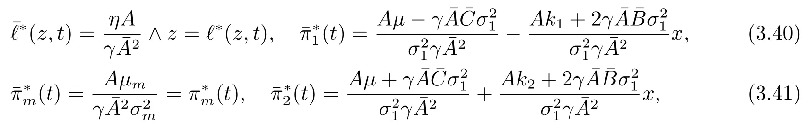
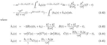
and the corresponding equilibrium value functionis

When Gu et al.[8]ignores mean reversion, we find that the equilibrium investment strategies given in Eqs.(3.40) and (3.41) are similar to that in Gu et al.[8], which considers the robust portfolio selection with the utility maximization.

Corollary 3.2 (Without Mispricing)In this case, we assume that the insurer ignores the mispricing between stock 1 and stock 2 in the market.If we don’t consider mispricing in our model, under the measure P, the wealth process becomes

The corresponding optimization problem becomes

Then, by some similar calculations, the equilibrium reinsurance-investment strategyis given by

and the corresponding equilibrium value function V2(t,w,y) is

We find that the equilibrium investment strategies given in eqs.(3.48) and (3.49) are similar to that in Zeng et al.[2], if Zeng et al.[2]considers the impact of delay on the optimal strategies.

4 Numerical Simulations

In this section, we supply some numerical examples to explain the effects of model parameters on the equilibrium investment strategy and utility losses from ignoring jump risk and mispricing.We suppose that the jump size Y1ifollow exponential distribution with parameter λY1, i.e., the density functions of Y1iis given by g(y1) = λY1exp{−λY1(y1+1)},y1≥ −1.Throughout the numerical analyses, unless otherwise stated, the basic parameters are given by β1= λY1= 1, r = 0.03, µ = 0.05, σ1= 0.3, θ = 0.2, η = 0.1, γ = 1, h = 0.5,δ =1.5 k1=0.2, k2=0.6, w =1, T =4, t=0.

4.1 Sensitivity Analysis of the Equilibrium Investment Strategy

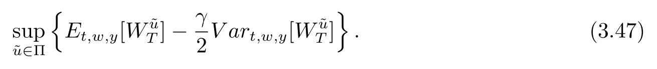
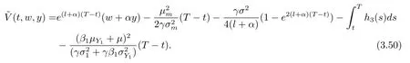
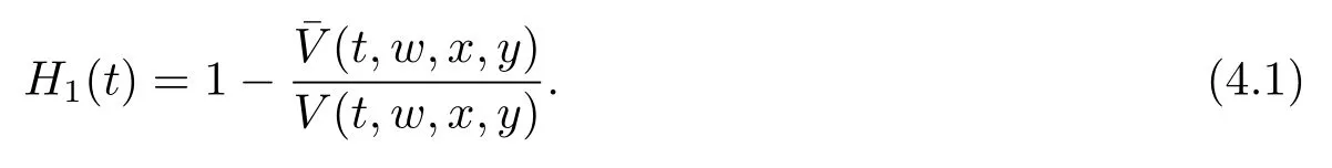
Figure 1 provides a sensitivity analysis of the mispricing x, the delayed parameter h,jump intensity β1and parameter λY1of the jump’s distribution function of these two stocks’s price processes for the equilibrium investment strategyi=1,2 .

In parts (a) of Figure 1, we find thatdecreases w.r.t. β1and increases w.r.t. λY1.This is because when β1becomes larger, the intensity of the jump in the first stock’s price process becomes stronger and the first stock becomes higher,so the money is invested in the first stock becomes less.At the same time, when λY1becomes larger, the mean and variance of Y1ibecome smaller.Therefore,under the same risk tolerance,the insurer will invest more in the first stock.In parts (b) of Figure 1, forthe analysis about it is similar to

In part (d) of Figure 1, we find that when the retention level π2(t) becomes smaller,the delayed horizon h becomes smaller.In part (c) of Figure 1, we find thatdecreases w.r.t. x andincreases w.r.t. x.In other words, as mispricing increases, the insurer will reduce their investment in stock 1 and increase their investment in stock 2.

4.2 Sensitivity Analysis of the Utility Loss Functions

In this subsection, we discuss the utility loss that can be caused when jump risks and mispricing are ignored for the insurer.

For equity but without loss of generality,we assume that the appreciation and volatility rates of stocks without jumps are the same as those with jumps, i.e., µY1i|nojump= µ +β1E[Y1i]and

So, the utility loss that ignores jump risks is defined as

As shown in (a) of Figure 2, we find that the utility loss increases w.r.t.the remaining time T − t and the effect of the remaining time T − t on the utility loss H1(t) is significant.

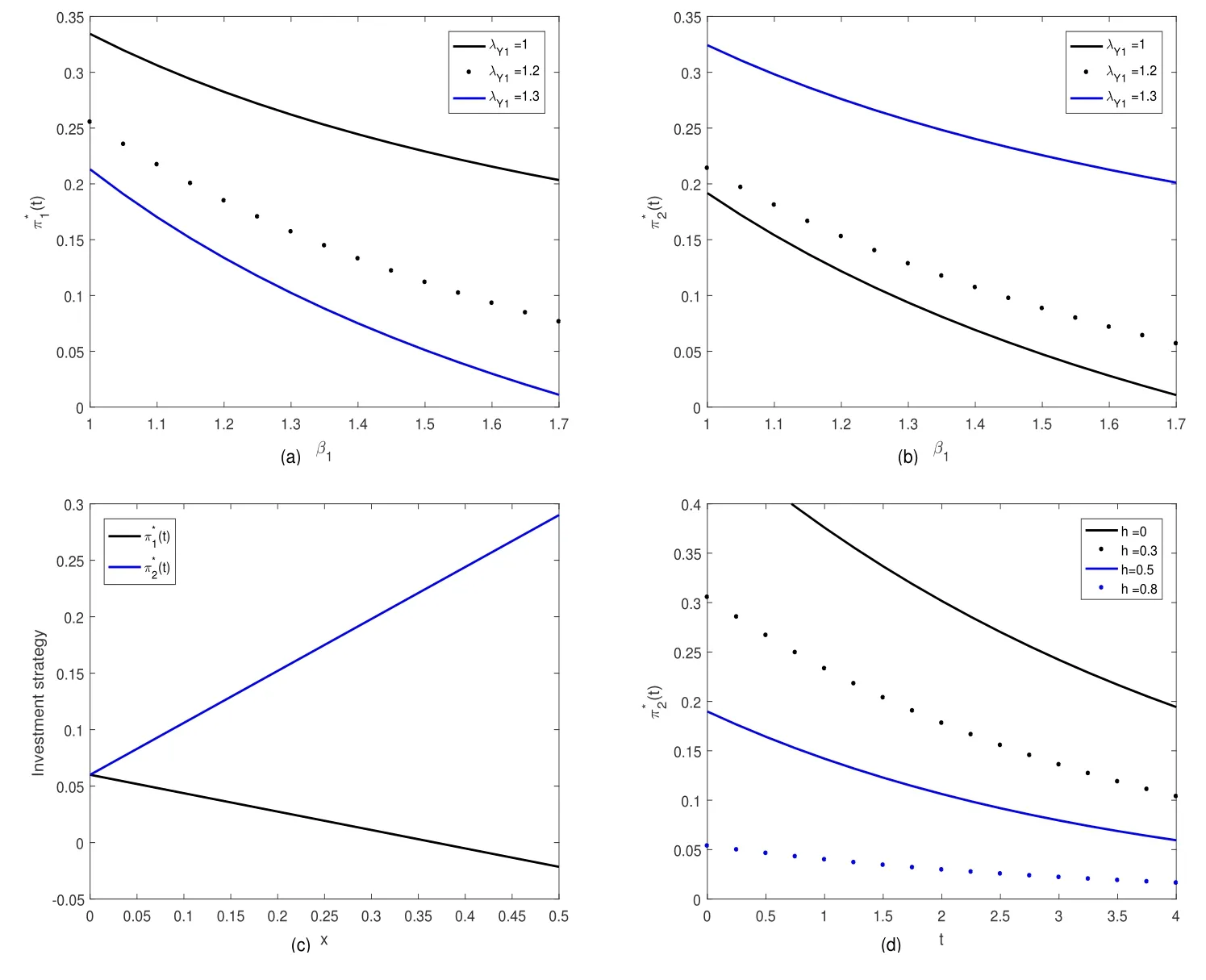
Figure 1 The effects of parameters on the equilibrium investment strategy

Figure 2 The effects of parameters on the utility loss functions

Then, we discuss the utility loss that can be caused when the mispricing is ignored for the insurer.The utility loss that ignores mispricing is defined as

From (b) of Figure 2, we can see that when the remaining time T −t increases, the utility loss H2(t) will also increase.And when T −t=0.3, we can find that the loss utility is less than 10%, however, when T −t = 4, we can find that the loss utility is more than 80%.This means that taking advantage of mispricing is more important for long-horizon investors than that for short-horizon investors.