WEAK AND STRONG DYADIC MARTINGALE SPACES WITH VARIABLE EXPONENTS
2020-03-14ZHANGChuanzhouWANGJiufengZHANGXueying
ZHANG Chuan-zhou, WANG Jiu-feng, ZHANG Xue-ying
(College of Science, Wuhan University of Science and Technology, Wuhan 430065, China)
Abstract: In this paper, we study the atomic decompositions of weak and strong dyadic martingale spaces with variable exponents.By atomic decompositions, we prove that sublinear operator T is bounded fromto wLp(·); Cesro operator is bounded from Hp(·) to Lp(·) and from Lp(·) to Lp(·), which generalize the boundedness of operators in constant exponent case.
Keywords: atomic decompositions; variable exponents; Cesro operator
1 Introduction
It’s well known that variable exponent Lebesgue spaces have been got more and more attention in modern analysis and functional space theory.In particular, Fan and Zhao [1]investigated various properties of variable exponent Lebesgue spaces and Sobolev spaces.Diening [2,3]and Cruz-Uribe [4]proved the boundedness of Hardy-Littlewood maximal operator on variable exponent Lebesgue function spaces Lp(·)(Rn) under the conditions that the exponent p(·) satisfies so called log-Hlder continuity and decay restriction.Many other authors studied its applications to harmonic analysis and some other subjects.
The situation of martingale spaces is different from function spaces.For example, the good-λ inequality method used in classical martingale theory can not be used in variable exponent case.However, recently, variable exponent martingale spaces have been paid more attention too.Aoyama [5]proved that, if p(·) is F0-measurable, then there exists a positive constant c such thatNakai and Sadasue[6]pointed out that the inverse is not true,namely,there exists a variable exponent p(·)such that p(·)is not F0-measurable, and the above inequality holds, under the assumption that every σ-algebra Fnis generated by countable atoms.Zhiwei Hao [7]established an atomic decomposition of a predictable martingale Hardy space with variable exponents defined on probability spaces.Motivated by them, we research dyadic martingale Hardy space with variable exponents.
2 Preliminaries and Notations
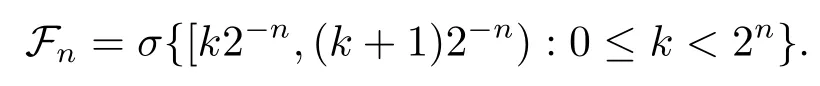
In this paper the unit interval [0,1) and Lebesgue measure P are to be considered.Throughout this paper, Z, N denote the integer set and nonnegative integer set.By a dyadic interval we mean one of the form [k2−n,(k+1)2−n) for some k ∈ N,0 ≤ k < 2n.Given n ∈ N and x ∈ [0,1),let In(x)denote the dyadic interval of length 2−nwhich contains x.The σ-algebra generated by the dyadic intervals {In(x) : x ∈ [0,1)} will be denoted by Fn, more precisely,
Obviously, (Fn) is regular.Define F = σ(∪nFn) and denote the set of dyadic intervals by A(Fn) and write A = ∪nA(Fn).The conditional expectation operators relative to Fnare denoted by En. For a complex valued martingale f =(fn)n≥0, denote dfi=fi− fi−1(with convention df−1=0) and

Remark 2.1(see [8]) If (Fn) is regular, then for all nonnegative adapted processesthere exist a constant c>0 and a stopping time τλsuch that

Let p(·) : [0,1) → (0,∞) be an F-measurable function, we define= ess inf{p(x) :x ∈ B},= ess sup{p(x) : x ∈ B}, B ⊂ [0,1). We use the abbreviationsand

when d(x,y)≤1/2.
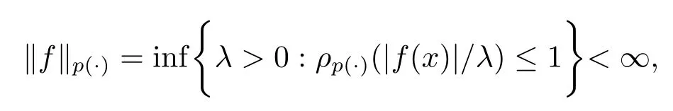
The Lebesgue space with variable exponent p(·) denoted by Lp(·)is defined as the set of all F-measurable functions f satisfying
If f =(fn) is a martingale, we define
Remark 2.2(see [7]) If p is log-Hlder continuous, then we have

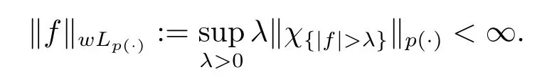
The weak Lebesgue space with variable exponent p(·) denoted by wLp(·)is defined as the set of all F-measurable functions f satisfying
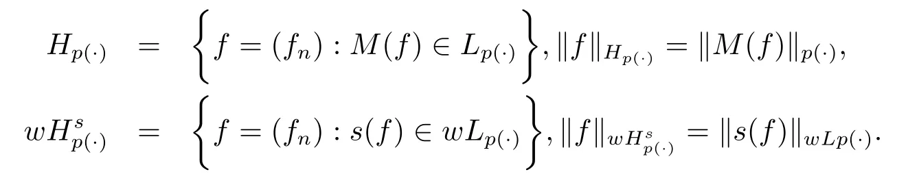
Then we define the strong and weak variable exponent dyadic martingale Hardy spaces as follows
We always denote by c some positive constant, but its value may be different in each appearance.
3 Weak Atomic Decompositions
Definition 3.1A measurable a is called a weak- atom if there exists a stopping time ν such that
(1) En(a)=0,n ≥ ν,

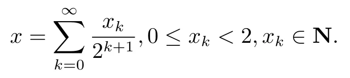
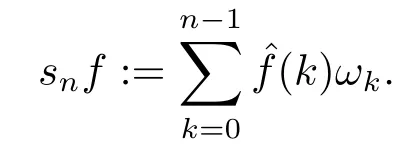
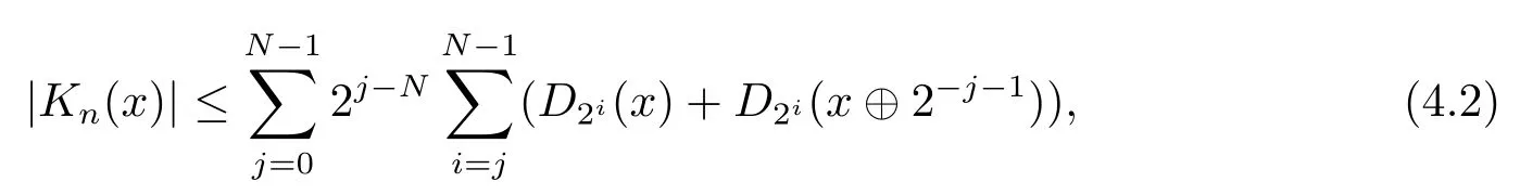
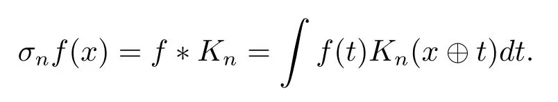
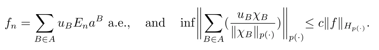
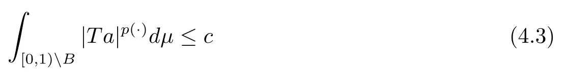
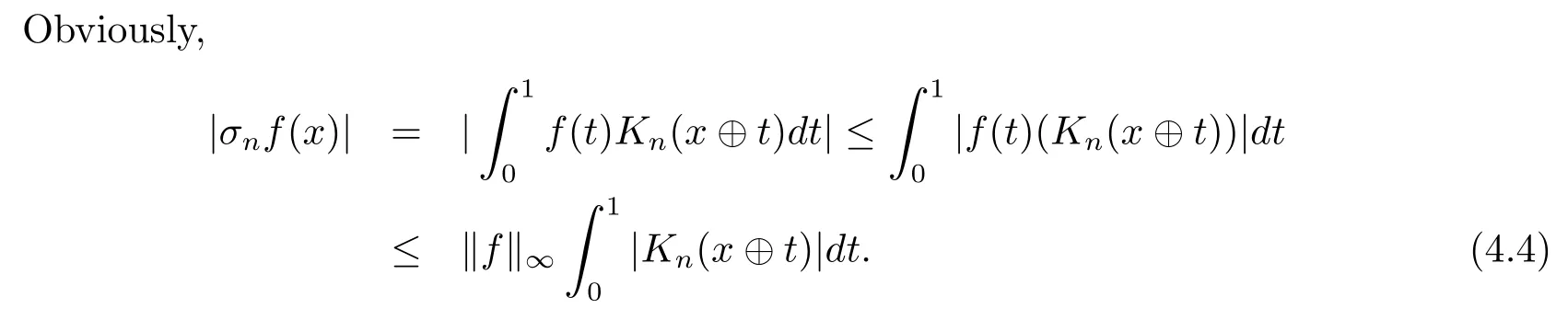
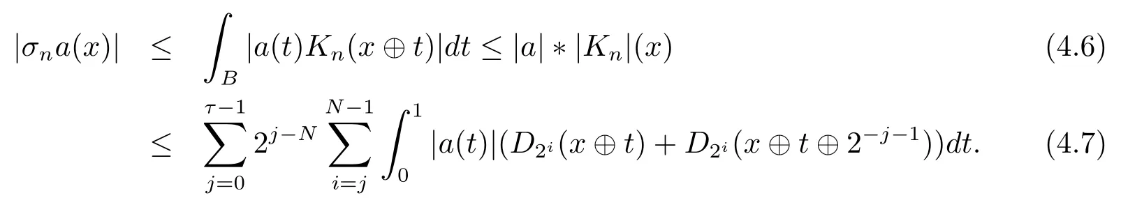
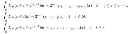
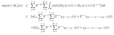
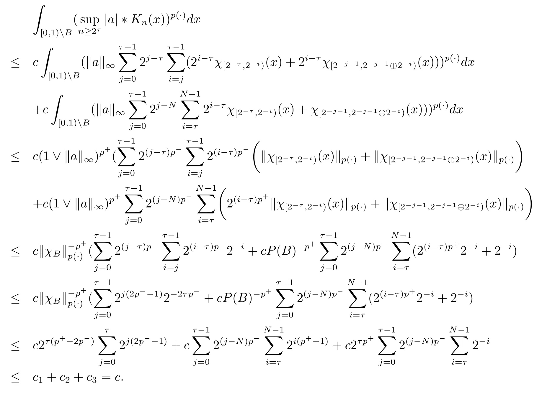
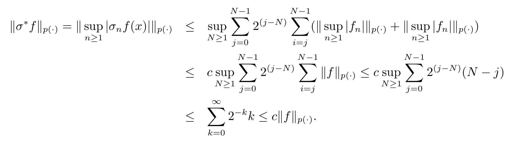
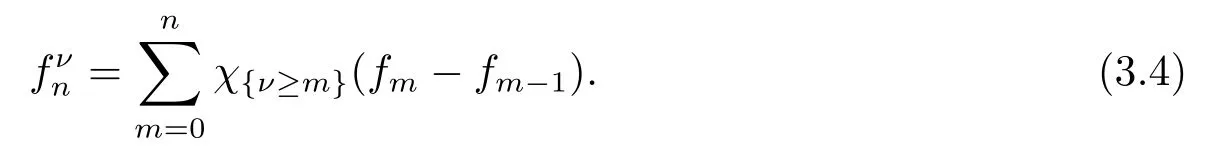
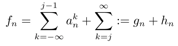
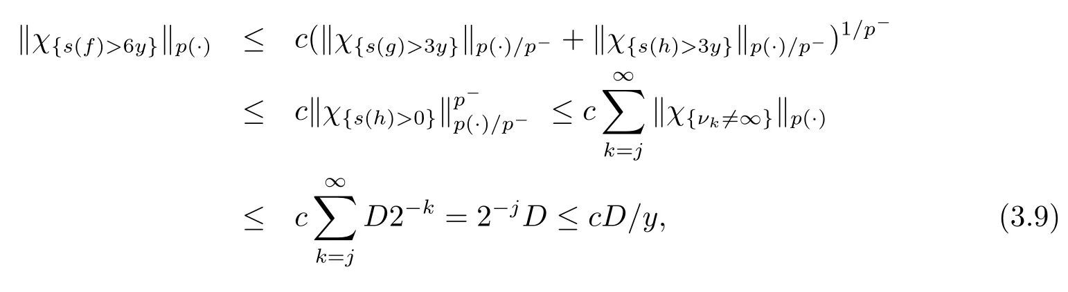
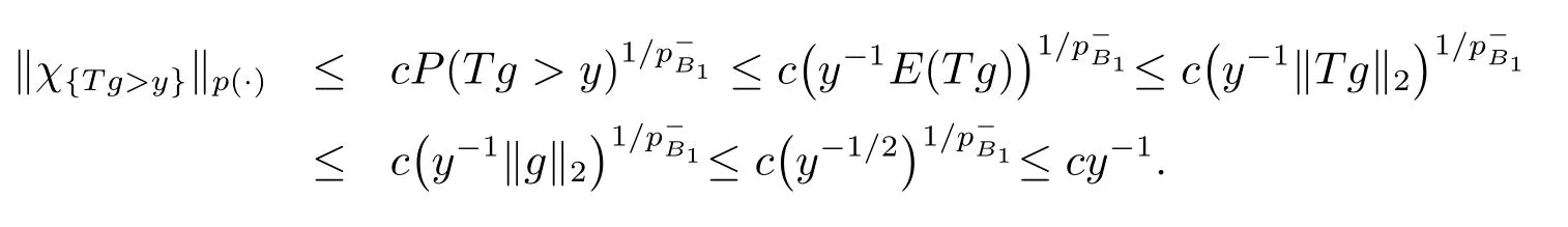
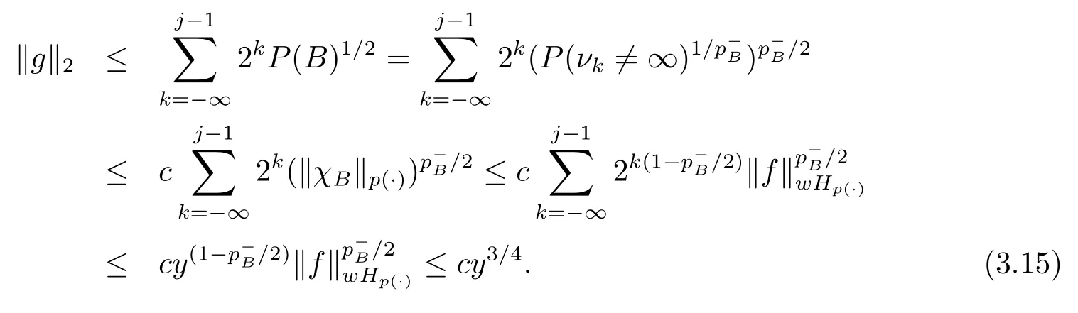
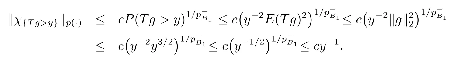
Theorem 3.2Suppose that p is log-Hlder continuous and 0 where the infimum is taken over all preceding decompositions of f. ProofAssume thatLet us define the stopping times νk:=inf{n ∈N:sn+1(f)>2k}. Consequently, fncan be written as Thus and p(·)/p−≥ 1 implies that s(f)≤ s(g)+s(h) and Since s(ak)≤3·2k, thus we get and so {s(g)>3y}⊂ {s(g)>3·2j}= ∅. which implies Thus we complete the proof. Theorem 3.3Suppose that p is log-Hlder continuous, 1/2 < p−≤ p+≤ 1 and suppose that sublinear T is bounded from L2to L2. If for all weak atom a supported on the interval I, then ProofWe may supposeTaking the atomic decomposition and the martingales g and h given in the proof of Theorem 3.2 we get that for any given y >0, (I) If 0 Define B1={Tg >y}, thus we have (II) If y >1. Thus We also have Combining (3.15) and (3.17) we get On the other hand, let B2={Tak>0}, Ikis support of ak, we have which implies By (3.18) and (3.19), we have Thus we complete the proof of Theorem 3.3. First we introduce the Walsh system.Every point x ∈[0,1) can be written in the following way In case there are two different forms, we choose the one for which For x,y ∈ [0,1) we definex ⊕ y =which is also called dyadic distance. The product system generated by these functions is the Walsh system: ωn(x) := If f ∈L1[0,1), then the numberis said to be the n-th Walsh-Fourier coefficient of f. Denote by snf the n-th partial sum of the Walsh-Fourier series of a martingale f,namely, Recall that the Walsh-Dirichlet kernelssatisfy Moreover,for any measurable function f,the sequence{f ∗D2n=s2nf =fn}is a martingale sequence. where x ∈ [0,1),n,N ∈ N,2N−1≤ n<2N(see [9]). Moreover, For n ∈N and a martingale f, the Cesro mean of order n of the Walsh-Fourier series of f is given by It is simple to show that in case f ∈L1[0,1) we have Definition 4.1A pair (a,B) of measurable function a and B ∈ A(Fn) is called a p(·)-atom if (1) En(a)=0, (2) Lemma 4.2(see [10]) Suppose that p is log-Hlder continuous and 0 < p−< p+≤ 1.For any f =(fn) ∈ Hp(·), there exist (aB,B)B∈Aof p(·)-atoms and (uB)B∈Aof nonnegative real numbers such that Lemma 4.3(see[10]) Suppose that the operator T is sublinear and for each p0 for every p(·)-atom (a,B).If T is bounded from L∞to L∞, then Theorem 4.4Suppose that p is log–Hlder continuous and 1/2 ProofBy Lemma 4.3, Theorem 4.4 will be complete if we show that the operator σ∗satisfies (4.3) and is bounded from L∞to L∞. Moreover for 2N−1≤ n<2Nand n>2τ(which implies N − 1 ≥ τ), Since x ∈[0,1)B, we have By the definition of an atom, for n ≥ 2τ,2N−1≤ n<2N, we have To verify(4.3)we have to investigate the integral of(supn|a|∗|Kn|(x))p(·)over[0,1)B.Integrating over [0,1)B, we obtain By Lemma 4.3 , the proof is completed. Theorem 4.5Suppose that p is log-Hlder continuous and 1 ProofWe assumeIf else, we let f replaced bySince where x ∈ [0,1),n,N ∈ N,2N−1≤ n<2N.Thus we have Thus by Doob’s inequality of variable exponents martingale spaces , we have Thus we complete the proof.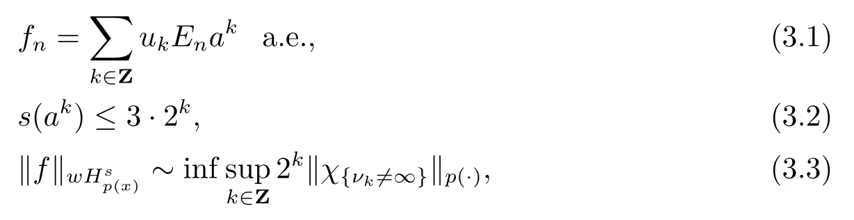


4 Boundedness of Cesro Operator