Joint 2D DOA and Doppler frequency estimation for L-shaped array using compressive sensing

WANG Shixin,ZHAO Yuan,LAILA Ibrahim,XIONG Ying,WANG Jun,and TANG Bin

School of Information and Communication Engineering,University of Electronic Science and Technology of China,Chengdu 611731,China

Abstract: A joint two-dimensional (2D) direction-of-arrival (DOA)and radial Doppler frequency estimation method for the L-shaped array is proposed in this paper based on the compressive sensing(CS) framework. Revised from the conventional CS-based methods where the joint spatial-temporal parameters are characterized in one large scale matrix, three smaller scale matrices with independent azimuth, elevation and Doppler frequency are introduced adopting a separable observation model. Afterwards, the estimation is achieved by L1-norm minimization and the Bayesian CS algorithm. In addition, under the L-shaped array topology, the azimuth and elevation are separated yet coupled to the same radial Doppler frequency. Hence, the pair matching problem is solved with the aid of the radial Doppler frequency. Finally, numerical simulations corroborate the feasibility and validity of the proposed algorithm.

Keywords: electronic warfare, L-shaped array, joint parameter estimation, L1-norm minimization, Bayesian compressive sensing(CS),pair matching.

1.Introduction

Joint direction-of-arrival (DOA) and Doppler frequency estimation have been applied in various fields including radar, sonar, communication and so on. Many DOA estimation algorithms have been proposed in the last decades,among which the subspace-based methods are the most popular ones, such as the multiple signal classfication method (MUSIC) [1], estimating sign parameters via rotational invariant technique (ESPRIT) [2] and other improved algorithms including root-MUSIC [3], total least squares–ESPRIT (TLS-ESPRIT), QR TLS-ESPRIT algorithm [4] as well as a combined ESPRIT-MUSIC approach[5].Additionally,in recent years,compressive sensing (CS) based DOA estimations have been reported taking advantages of the spatial sparsity of the signals,which can accurately obtain DOA estimation with only a few samples. Especially, the reconstruction methods are well addressed.For example,this problem was solved through orthogonal matching pursuit(OMP)and compressive sampling matching pursuit (CoSaMP) in [6] and [7]. On the other hand, theL1-norm minimization method was proposed in [8] with stability at a low signal to noise ratio(SNR). Moreover, the Bayesian CS algorithm was proposed in[9,10],showing a promising prospect with its accurate DOA estimation performance.

In this paper, we exploit the L-shaped array to implement the joint two-dimensional (2D) DOA and radial Doppler frequency estimation. Actually, some methods have been proposed to solve this estimation problem.For example, the 2D-MUSIC algorithm [11] and the multi-ESPRIT algorithm[12]were adopted to solve the joint estimation problem for coprime arrays.However,these algorithms need a large amount of sampled data to ensure the accuracy and validity.To solve the limitation, Dang et al.[13] resorted a CS-based method to obtain DOA estimation,then the short-time Fourier transform(STFT)was applied to capture the Doppler frequency using the time window.Nevertheless,this method did not utilize the property that the Doppler frequency is sparse in nature for the moving platform (fighter plane, missile and so on) reconnaissance.In[14],the authors exploited an algorithm based on sparse Bayesian learning (SBL) to obtain the joint DOA and Doppler estimation.Like other conventional CS-based methods,the joint spatial-temporal parameters are characterized in one large scale matrix, which will, in turn, increase the computing burden.Fortunately, Luo et al. [15]proposed a separable observation model,which splited the observation matrix into two small matrices. With the aid of this separable observation framework, we separate the joint spatial-temporal observation matrix into three individual small matrices under the L-shaped array. Further,we extend the joint DOA and Doppler frequency estimation to the three-dimensional(3D)scenario.

The novelty of this paper can be summarized as follows:(i)we achieve a joint estimation under the CS framework; (ii) we solve the DOA pair matching problem under the L-shaped array topology. To this aim, we resort to theL1-norm minimization to estimate the azimuth and the elevation stably at a low SNR. Moreover, we exploit the Bayesian CS theory to estimate the radial Doppler frequency accurately.Although the azimuth and elevation are estimated separately, they are coupled to the same radial Doppler frequency,so the method can also implement pair matching.

The rest of this paper is organized as follows.Section 2 formulates the signal models. In Section 3, the proposed method is described in detail.Section 4 presents our simulation through numerical Monte-Carlo experiments. Section 5 draws some conclusions.

2.Signal models

Suppose an L-shaped array constructed by two orthogonal uniform linear arrays (ULA) in thex-yplane, as is illustrated in Fig. 1. DenoteMby the amount of antenna in each sub-array. Moreover, in this paper, we follow the definition in [16]that the elevationθrepresents the angle betweenokand they-axis, the azimuthϕrepresents the angle betweenokand thex-axis.

Fig.1 Configuration of an L-shaped array

Suppose that there areKuncorrelated far-field narrowband signals impinging on the L-shaped array from different directions. Under the geometry shown in Fig. 1, the received signals collected by the ULAs along thex-axis andy-axis can be respectively written as

where the incident signal vector and the receiving additive white Gaussian noise(AWGN)for ULAs along thex-axis andy-axis can be expressed as

and the manifold along thex-axis andy-axis is expressed as

whose elements,i.e.,the steering vectors,are calculated by

wherek= 1,2,3,...,K;αk= 2πdcosθk/λandβk=2πdcosϕk/λ;d=λ/2 is the interspace between adjacent antennas;λ=c/f0is the transmitted signal wavelength;[ ]Tis the transpose operator;f0is the carrier frequency.Fortunately, the estimation of this carrier frequency has been addressed in[17].Therefore,in this paper,we assume the carrier frequency estimation has been accomplished for the sake of simplicity.

Let us first consider the ULA along thex-axis (the derivation for they-axis is symmetry),suppose the signal amplitude equals 1,thekth signal received by themth antenna can be expressed as

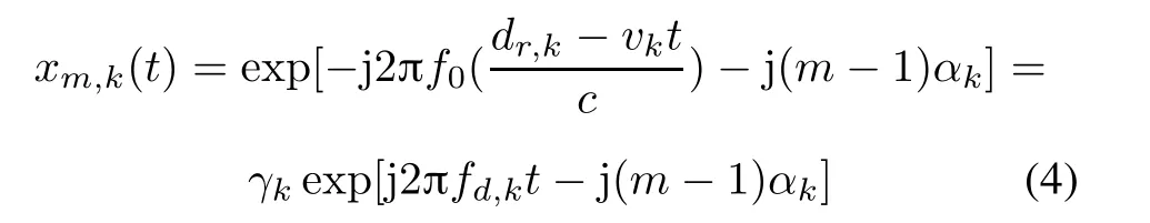
wherefd,kdenotes the radial Doppler frequency of thekth target,dr,kandvkstand for the initial radial distance and the radial velocity of thekth target,cis the speed of light,respectively.

Hence,the overall baseband signal received by themth antenna is given by

whereγk=exp(-j2πdr,k/λ)is a complex amplitude.We collect samples simultaneously from the signal with a stable sampling rateTssatisfying the Nyquist constraint,so as to form a data matrixX.For the derivation simplicity,we ignore the AWGN for time being,and the(m,l)th element of this data matrix can be written as

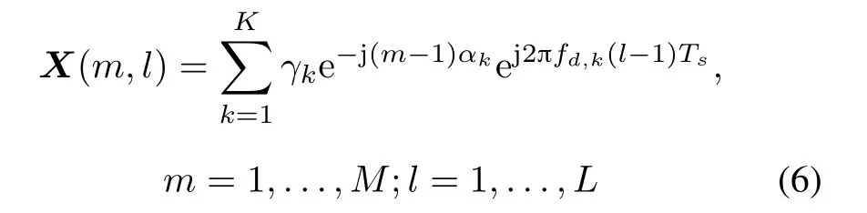
whereLdenotes the length of the snapshots.

We divide the azimuth and Doppler space on grids intoNandQgrids respectively.Then,we can define the observation matrixΦ ∈CM×NandF ∈CQ×Las

wherea(ϕk) (k= 1,2,...,N) inherits the definition as(3);is the Doppler frequency bin vector.Therefore,we can define anN×Qindex matrixSxwhose(i,j)th element can be expressed as

After the grid division,the following sparse representation for the signal model is provided as

Due to the fact that the number of targets is much smaller than the grid size of angles and Doppler frequencies (i.e.,N), the matrixSxis indeed a spatial-temporal sparse matrix,wherein the row sparsity of it determines the azimuth of the target and the column sparsity determines the radial Doppler frequencies of the target.AssumingSxisK-sparse (K < L), when right-multiplied with anLrank matrixF,the sparsity is still guaranteed,i.e.,we can introduce a row sparse transition matrixZx=SxF,whereZxshares the same sparsity as the matrixSx. Hence, (9)can be reformulated as

Therefore,the index of the non-zero rows of the matrixZxdetermines the azimuth of the target.

Similarly,the elevation space can be expressed as

whereΘ ∈CM×N.The data matrix received by the ULA along they-axis can be formulated as

and the corresponding transition matrix is given byZy=SyF.

Therefore,the estimation of the 2D DOA is now equivalent to search for the non-zero rows of transition matricesZxandZy. We can then estimate the Doppler frequency by searching for the non-zero columns of sparse matricesSxandSy.Also,thanks to the separable observation model, we can divide the azimuth/elevation-Doppler frequency space intoNgrids separately instead of anN2grids large scale space matrix.

3.Proposed joint estimation algorithm

With analysis above,we can achieve our DOA estimation goal by first reconstructing the transition matrixZxand retrieving the sparse matrixSx, thereafter. These two steps can both be categorized as the multiple measurement vector (MMV) problems in the CS theory.Many approaches have shown a superior capability to solve this MMV problem, including the multiple OMP (M-OMP) algorithm[18], multiple focal under-determined system solver (MFOCUSS) algorithm[19],L1-norm minimization and the multitask-Bayesian CS(MT-BCS)[20].However,most of these methods suffer from a performance digression when the SNR is low.This estimation error will bring failure to our further Doppler frequency estimation. Therefore, we can first resort toL1-norm minimization,which has a superior performance in the noisy environment.The MT-BCS algorithm is then followed by the computational efficiency.This algorithm shows an outstanding accuracy when the first step brings less residual into the radial Doppler frequency estimation.

3.1 Joint 2D DOA and radial Doppler frequency estimation

SinceZxshares the same row sparsity property as the matrixSx, and the index of the non-zero rows of the matrixZxdetermines the azimuth angles of the target. We resort to theL1-norm minimization,where reconstructingZxfrom(9)can be converted into the following optimization problem[8]:

whereis thenth row ofand‖ · ‖2denote the Frobenius norm,L1norm andL2norm respectively.μis the regularization parameter,which controls the relative importance applied to the error and the sparseness term, and one can chooseμsuch that(see Section V in[8]for more details).

Since OP1 in (13) contains a term, which is neither linear nor quadratic,so we turn to the second-order cone(SOC)programming[21],which is a suitable framework for the objective function.Moreover,the main reason for considering SOC programming instead of generic nonlinear optimization for our problem is the availability of efficient interior point algorithms for the numerical solution of the former[8].

We defineZx{l}as thelth column of the matrixZx.OP1 is then formulated as an SOC programming problem,i.e.,OP2(see the Appendix in[8]for more details).

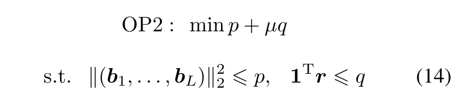
wherebl=X{l} - ΦZx{l}(l= 1,2,...,L),‖Zx[n]‖2≤rn(n= 1,2,...,N);p,qandr ∈CN×1are the introduced auxiliary variables;X{l}represents thelth column of the matrixX. Then we can use the convex optimization(CVX)[22]toolbox in Matlab to reconstruct the matrixZx.

Recall thatZx=SxF,whereSxis the sparse matrix,the index of the non-zero elements inSxcorrespond to the estimation of the azimuth angles and the radial Doppler frequencies;Fis the observation matrix.We take the transpose of the sparse matrixZx,then we can obtain

Further,we utilize the MT-BCS algorithm to reconstruct the sparse matrixSx.

Introducing the auxiliary matricesand(15) can be reformulated asSince the MT-BCS approach cannot process complex data directly,we use the following real data model:

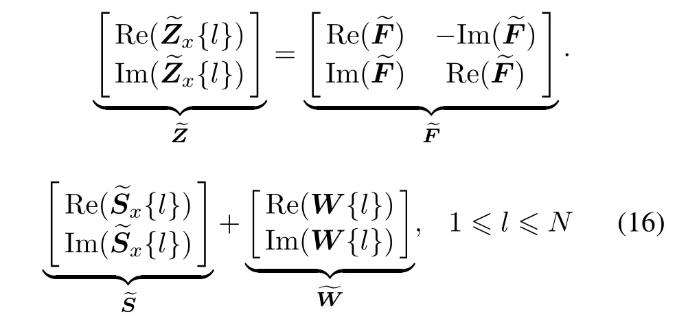
where Re(·) and Im(·) denote the real and imaginary operator,respectively;W{l}stands for thelth column of the noise matrix with unknown variance.

According to the MT-BCS theory, the column vector of the sparse matrix is obtained by the probability density function way by solving the following[23]optimal problem,i.e.,OP3,given by

whereIdenotes theN×Nidentity matrix,aandbare defined by the users[24].Finally,the retrieved sparse matrix[23]turns out to be

In addition, we substitute the signal azimuth measurement matrix into(8).The elevation angle observation matrixΘcan obtain the baseband discrete signal model received by the ULA along they-axis,which is illustrated in(12). Similarly, the row sparse matrixZyand the sparse matrixSycan be obtained by the way we mentioned above.

3.2 2D DOA pair matching based on the radial Doppler frequency

As is stated in Section 3.1, we estimate the azimuth and elevation separately,so pair matching is required after the 2D DOA estimation[16,25].Fortunately,we can solve this problem by utilizing the evidence that for the same target,the azimuth and elevation angles are coupled with the same radial Doppler frequency.

We define two sets to denote the 2D DOA and radial Doppler frequencies by

The pair matching problem can be illustrated as Fig.2,where the “distance” between theith element inand thejth element inis defined asdij=|fxi-fyj|.The solid line means the matched azimuth-elevation-Doppler frequency and the dash line means unmatched ones.

We further assume different targets have different Doppler frequencies. Then for a fixed azimuth indexi=1,...,K,the specific pair matching procedure is to repeat the following minimization forj=1,...,K.

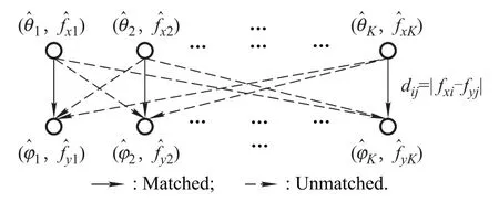
Fig.2 Demonstration of pair matching

InputThe DOA-radial Doppler frequencies pair setsand

Loopfori=1 toKdo

(i)Calculate the frequency offset using(23);

End loop.

Finally, (ϕi,θjopt) is matched wherei=1,...,K;jopt=1,...,K.

3.3 The proposed DOA and Doppler frequency estimator

According to the above process, we can implement the joint 2D DOA and the radial Doppler frequency estimation.In addition,we notice that some preprocessing needs to be done on matricesZxandZyto reduce the calculation burden.Delete the rows with small energy and reserve theKrows with strong energy,define new matrices asZxminandZymin, then plugZxminandZymininto (13). Note that all the reserved row indices should be recorded as the results of the azimuth and elevation angles estimation.

In summary,with the signal matrixX,observation matrixΦand matrixF, the pseudo code of the proposed algorithm is illustrated as follows.

InitializationConstruct the observation matricesΦ,ΘandF.

Estimation of DOA:

(i)Convert(13)into an SOC programming problem.

(ii) Use the CVX toolbox in Matlab to reconstruct the matricesZxandZy.

Estimation of radial Doppler frequency.

(iii)Using(16)to convert(15)to the real data model.

(iv)Calculate the likelihood functionΨ(α)using(19),where theCMT-BCS is given by(20).

(vi)Finally,reconstruct the matrixSxandSyby using(21).

Pair matching for DOA.

(vii)Calculate the function(23)repeatedly,until all the azimuth and elevation angles are matched.

3.4 Complexity analysis

In this part, we analyze the computational complexity of the proposed approach and the traditional CS-based estimation approach. SALARI et al. [14] solved the onedimensional(1D)DOA and Doppler frequency estimation,and the scale of the basis matrix is supposed asML×NQ,the computational complexity of the traditional CS-based approach isO(N3Q3).If this approach is extended to the 3D scenario, the computational complexity is increased with it. For the proposed approach, the scale of the basisΦisM×N,ofFisQ×L,so the complexity for solving the data received by ULA along thex-axis isO(N3+Q3).Similarly, the scale of the basisΘisM × N, the complexity for solving the data received by ULA along theyaxis is alsoO(N3+Q3), and the overall complexity isO(N3+Q3).

4.Performance evaluation

In this section, we describe some numerical results obtained by Monte-Carlo simulation. To be specific, an L-shaped array illustrated in Fig.1 is considered,the interval between each antenna is half-wavelength. Moreover,we assume two uncorrelated far-field narrowband signals impinge on the L-shaped array, and their 2D DOA and radial Doppler frequencies are set to be [ϕ1,θ1,fd1] =[3°,7°,260 Hz]and[ϕ2,θ2,fd2]=[4°,7.5°,320 Hz].The SNR is defined as 10·lg(η/σ2), whereηis the signal power,σ2is the noise power,respectively.θ,ϕ ∈(0°,10°)and the direction is divided uniformly intoN= 101 grids with the interval equal to 0.1°.fd ∈(250 Hz,350 Hz)and the radial Doppler frequency is also divided intoQ=101 grids with the interval equal to 1 Hz.

Additionally, in all simulations, 200 independent runs are conducted to calculate the root mean square error(RMSE)of the 2D DOA and Doppler frequency as

whereTdenotes the number of Monte Carlo experiments,Kdenotes the total number of targets,anddenote the estimated values of thekth target at theith Monte Carlo experiment,respectively.

Simulation 1Demonstration of the parameter estimation process

In this simulation, we demonstrate the estimation procedure.To this end,we set SNR to be 20 dB,the amount of antennas is 10, and the length of snapshots is 50.Fig. 3(a) and Fig. 4(a) show the spectra ofZxandZyrespectively. It can be observed that the energy concentrates on the actual angles. Fig. 3(b) and Fig. 4(b) show the spectra ofSxandSyrespectively,which have the distinct peaks corresponding to the sparse distribution on the spatial-temporal domain.

Fig.3 Spectra of sparses matrix about x-axis

Fig.4 Spectra of sparses matrix about y-axis

Simulation 22D DOA and radial Doppler frequency estimation performance evaluation

In this simulation, we evaluate the estimation performance with respect to SNR and it can be easily observed from Fig.5 and Fig.6 that the accuracy of DOA and radial Doppler frequency estimation improves with the increase of the SNR.

Fig.5 RMSE of DOA/radial Doppler frequency versus SNR and M

Fig.6 RMSE of DOA/radial Doppler frequency versus SNR and L

Specifically,in Fig.5 we investigate estimation performance as a function ofM.To this aim,the length of snapshots is fixed at 50.It is observed that with increasingM,the DOA estimation performance is noticeably improved.It is also observed by comparing the two sub-figures that,the number of antennas has a less effect on the Doppler frequency estimation performance than that on the DOA estimation performance. This phenomenon is brought by the fact that, in the proposed method, the Doppler frequency estimation performance is influenced by the length of the snapshots, which is fixed in this simulation; and the row sparse matrixZxandZyareMrelated. Meanwhile,the estimation errors of the row sparse matrix have already been small.Hence,Mhas limited effect on the radial Doppler frequency estimation performance compared with the DOA estimation performance.

Likewise, in Fig. 6 we investigate estimation performance as a function ofL.To this aim,the amount of antennas is fixed at 12.Fig.6(b)indicates that the performance of the radial Doppler frequency estimation is significantly improved by increasing the length of snapshots.However,it is also observed by comparing the sub-figures that, the length of snapshots has a less effect on the DOA estimation performance than that on the Doppler frequency estimation performance.Similar to the reasons above,the DOA estimation performance is influenced by the number of the antennas,which is fixed in this simulation.Thus,Lhas limited effect on the DOA estimation performance compared with the Doppler frequency estimation performance.

Simulation 3Comparison with existing methods

Some simulations of joint DOA and Doppler estimation are compared with the proposed method in this paper.It is shown in Fig. 7 that the proposed method has better performance than other methods especially in low SNRs.

Fig.7 Comparison of performances

5.Conclusions

In this paper, a joint 2D DOA and radial Doppler frequency estimation method for the L-shaped array is proposed based on the CS theory.Resorting to the separable observation framework, the joint spatial-temporal observation matrix is separated into three individual small matrices, afterwards theL1-norm minimization method and the MT-BCS algorithm are used to estimate 2D DOA and radial Doppler frequencies respectively. Further, the pair matching problem can be solved since azimuth and elevation angles are coupled to the same radial Doppler frequency.The simulation results verify the effectiveness and superiority of the proposed method.

On the contrary,the estimation accuracy of the proposed algorithm depends on the grid scaleN. However, denser grids will increase the computation burden and vice versa.Therefore, refined dynamic grid meshing is to be developed. In addition, for the proposed pair matching algorithm,the optimal solution obtained from each iteration is actually a local optimal solution rather than a global optimal solution.Therefore,in future research,we will investigate a revised matching algorithm.Moreover,as is stated in most DOA estimate studies,since wide-band signals are applied more in practice,utilizing CS based DOA estimation to wide-band models will be another future research.