A Study on the Correlation Between Poles and Cuts in ππ Scattering∗

Ling-Yun Dai (戴凌云), Xian-Wei Kang (康现伟), Tao Luo (罗涛), and Ulf-G.Meißner

1School of Physics and Electronics, Hunan University, Changsha 410082, China

2College of Nuclear Science and Technology, Beijing Normal University, Beijing 100875, China

3Key Laboratory of Nuclear Physics and Ion-beam Application(MOE)and Institute of Modern Physics,Fudan University,Shanghai 200443, China

4Helmholtz Institut für Strahlen- und Kernphysik and Bethe Center for Theoretical Physics, Universität Bonn, D-53115 Bonn, Germany

5Institute for Advanced Simulation, Institut für Kernphysik and Jülich Center for Hadron Physics, Forschungszentrum Jülich, D-52425 Jülich, Germany

Abstract In this paper we propose a dispersive method to describe two-body scattering with unitarity imposed.This approach is applied to elastic ππ scattering.The amplitudes keep single-channel unitarity and describe the experimental data well, and the low-energy amplitudes are consistent with that of chiral perturbation theory.The pole locations of the σ, f0(980), ρ(770) and f2(1270) and their couplings to ππ are obtained.A virtual state appearing in the isospin-two S-wave is confirmed.The correlations between the left (and right) hand cut and the poles are discussed.Our results show that the poles are more sensitive to the right hand cut rather than the left hand cut.The proposed method could be used to study other two-body scattering processes.

Key words:dispersion relations, partial-wave analysis, chiral lagrangian, meson production

1 Introduction

In a two-body scattering system, for example two hadrons, the general principals that we know are unitarity,analyticity,crossing,the discrete symmetries,etc.The resonances that appear as the intermediate states in such system are important.Among them the lightest scalar mesons, related toππscattering, have the same quantum numbers as the QCD vacuum and are rather interesting,for some early references, see Refs.[1–3].Theππscattering amplitude is also crucial to clarify the hadronic contribution to the anomalous magnetic moment of the muon, see e.g.Refs.[4–5].To study the resonances in a given scattering process, one needs dispersion relations to continue the amplitude from the reals-axis (the physical region)to the complex-splane(see e.g.,Refs.[6–9])where the pole locations and their couplings are extracted.Following this method,some work on the light scalars can be found in Refs.[10–15], where the accurate pole locations and residues of theσandκmesons are given.

For the dispersive methods, a key problem is how to determine the left hand cut (l.h.c.) and the right hand cut (r.h.c.), with the unitarity kept at the same time.In Refs.[7–8]the l.h.c.is estimated by crossed-channel exchange of resonances, where chiral effective field theory(χEFT) is used to calculate the amplitude.And the contribution of r.h.c.is represented by an Omnés function,with unitarity kept.In the well-known Roy equations,crossing symmetry and analyticity are perfectly combined together as the l.h.c.is represented by the unitary cuts of the partial waves.The single channel unitarity is also well imposed by keeping the real part of the partial wave amplitudes the same as what is calculated by the phase shift directly, which could be obtained by fitting to the experimental data in some analyses.Until now, Roy and Roy-Steiner equations certainly give the most accurate description of the two-body scattering amplitude and the information of resonances appearing as the intermediate states, such asππ,πKscattering and the pole locations and residues of theρ,σ,f0(980) andκ, etc., see e.g.Refs.[13–15].In addition, Ref.[14]shows that the l.h.c.can not be ignored for the determination of the pole location of theσ.By removing the parabola term of the l.h.c.,theσpole location is changed by about 15% accordingly,while the unitarity is violated due to the removal of the l.h.c.And thus the method to get the poles on the second Riemann sheet, calculated from the zeros of the S-matrix,is not reliable any more, as the method is based on the continuation implemented by unitarity.Here,we focus on obtaining a quantitative relation between cuts and poles,with unitarity imposed and the l.h.c.and r.h.c.are correlated with each other.

This paper is organized as follows:In Sec.2 we establish a dispersive method based on the phase.In the physical region we also represent the amplitudes by an Omn`es function of the phase above threshold.In Sec.3 we fit theππscattering amplitudes up to 1 GeV in a model-independent way, including theIJ=00,02,11,20 waves, whereIdenotes the total isospin andJthe angular momentum.The fit results are the same as those given by the Omnés function representation and comparable with those of chiral perturbation theory (χPT) in the low-energy region.The poles and couplings are also extracted.In Sec.4 we give the estimation of the relation between poles and cuts, including both the l.h.c.and the r.h.c.We end with a brief summary.

2 Scattering Amplitude Formalism

2.1 A Dispersive Representation

The two-body partial wave scattering amplitude can be written as:

withφ(s) the phase andf(s) a real function.By writing a dispersion relation for lnT(s), one has:

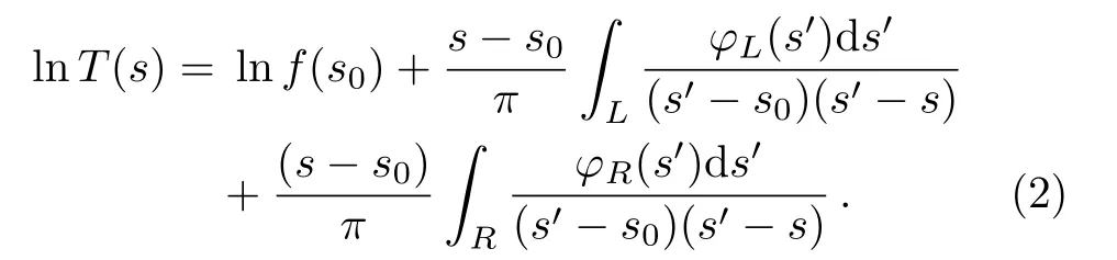
Here,s0is chosen at a specific point where the amplitude is real, and “L” denotes the l.h.c.and “R” stands for the r.h.c.The amplitude turns into

On the other hand, unitarity is a general principal required for the scattering amplitude.In the single channel case one has

wheresis in the elastic region andρ(s)is the phase space factor.Substituting Eq.(3) into Eq.(4), we obtain a representation (in the elastic region) for a single channel scattering amplitude

Also, the Omnés function of the phase[16]for the l.h.c.is correlated with that of the r.h.c.which is again valid in the elastic region.A simple way to get the two-body scattering amplitude proceeds in two steps:First, we follow Eq.(5) to fit the Omnés function of the r.h.c.to experimental data, and then use Eq.(6)and other constraints below the threshold to fit the Omnés function of the l.h.c.Note that Eq.(5)does not only work for the single channel case, but also for the coupled channel case in the physical region.

2.2 On ππ Scattering

In the equations above, the threshold factor is not included.Considering such factors, we need to change the amplitudes into:

Here and in what follows, we takeππscatering as an example.Thus one haszJI=4Mπ2for the P-, D-, and higher partial waves,andzIJis the Adler zero for the S-waves.nJis one for S- and P-waves and two for D waves.We define a reduced amplitude

and again we can write a dispersion relation for ln(s),so that we have

Here,s0could be chosen from the range[0,4M2π].For the r.h.c., we cut off the integration somewhere in the high energy region, see discussions in the next sections.We have

TheTIJ(s0) could be fixed byχPT or scattering lengths,or other low-energy constraints.For simplicity, we chooses0=0.Combining unitarity, embodied by Eq.(5), we have a correlation between Omnés functions of l.h.c.and r.h.c.in the elastic region

This is similar to Eq.(6).Substituting Eq.(11) into Eq.(10), we still have Eq.(5).Since we know theππscattering amplitudes well in the region [4M2π, 2 GeV2]andχPT describes the amplitudes well in the low-energy region, we have to fit the l.h.c.to both Eq.(6) andχPT.

3 Phenomenology

3.1 ππ Scattering Amplitudes

For theππscattering amplitude, we can parameterize the phase caused by the l.h.c.by a conformal mapping

with

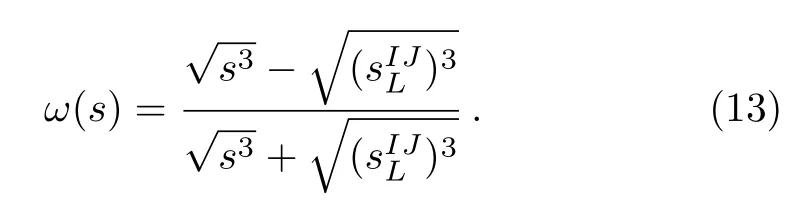
Notice that Imω(s)behaves asarounds=0,which is consistent with that ofχPT,see Ref.[12]and references therein.

As concerns the r.h.c., it is less known in the high energy region.However, these distant r.h.c.should have less important effects in the low-energy region, especially in the regions ≤1 GeV2.We choose three kinds ofΩIJR(s) to test the stability and uncertainty caused by the distant r.h.c.In Case A, the phases are cut off ats=2.25 GeV2.[7]In Case B, the phases are given by Ref.[7],up tos=22 GeV2.In Case C,the phases/Omn`es functions of the r.h.c.are given by Refs.[17–19]and references therein, up tos=22 GeV2.Here, the phases are fitted to the experimental data in Refs.[20–21]up t√o=2 GeV and constrained by unitarity up to=4 GeV.Notice that in Case A and B the phase of the isospin-one P-wave is given by CFDIV in Ref.[22],and we continue it to the higher energy region by means of the function

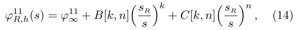
with

The function (and also its first derivative) is smooth at the pointsR.We setk=1,n=2,sR=1.42GeV2andφ11∞=160◦, which is close toφ11R((1.4 GeV)2)=170◦and ensures that the phase in the high energy region behaves smoothly.The upper limits of the integration of the r.h.c.of isospin-one P-wave are the same as the other partial waves.The three kinds of Omnes functions have different magnitudes.For example, in isospin zero S-wave the difference between Cases A/B and C is 17/6 percent ats=0.5 GeV2.And that is 2/17 percent for isospin one P-wave.

The parameters of our fits for all the Cases are given in Table 1.ThecIJnare determined by the following procedure.In the elastic region, we choose one or two “mesh points”, equaling to the number of the coefficientscIJn.Combining Eqs.(11) and (12), we can build a matrix and solve forcIJn.We adjust the “mesh points” andsIJLto make the solutions to be consistent with that of Eq.(5)in the physical region.For instance, we choose one “mesh point” ass1=0.7 GeV2in Case A, and two points ass1=0.2 GeV2ands2=0.6 GeV2in Cases B and C.Other partial waves are treated similarly.Note that we do not choose more mesh points, as the correlation between each terms of dispersion relation will become stronger and we will have larger number ofcIJn, resulting in more twisted amplitudes.This strategy gives a good description of the amplitudes, with unitarity kept.See the fit results shown in Fig.1.Here all the partial waves refer to Case B,in which the phase is cut off ats=2.25 GeV2.The amplitudes from the other Cases are quite close to this one, except for the inelastic region and the distant l.h.c.(≤−0.4 GeV2).Our fit, both the real part (black solid line) and imaginary (black dotted line) part of the amplitudes shown in Fig.1, is indistinguishable from that given by the K-Matrix[7]or CFDIV.[22]Note that the amplitudes given by Eq.(5) are exactly the same as those of the K-Matrix or CFDIV fromππthreshold to the inelastic threshold.This implies that the unitarity is respected.To test it quantitatively, we define

∆TIJ(sn)is the difference between our amplitude and that of Eq.(5).We use this equation to refine our solutions,that is, theand “mesh points” are selected out to makesmall.Here we choosesn=(0.1–0.9) GeV2for the S-waves,sn=(0.1–0.8) GeV2for the P-wave,andsn=(0.1-1.0) GeV2for the D-wave, with step of 0.1 GeV2.These points are located between theππand the inelastic thresholds.From here on all the steps are chosen to be 0.1 GeV2(or 0.1 GeV for).We find thatand=1.4%.The violation of unitarity is rather small at elastic region.Notice that if we remove out the Omnes function of the right hand phase, only the l.h.c.part(timesT(0)) remains and it is a smooth real function aboves >0.Since the contribution of the l.h.c.is determined rather well in the elastic region, it would be natrual to keep working well not faraway from the inelastic threshld.This is why the amplitudes could be described well up to 1.2 GeV for S- and P-waves.These are enough for us to discuss the poles and cuts ofσ,ρandf0(980).

ForTIJ(0),χPT could be used to fix it.The analytical SU(3) 1-loopχPT amplitudes of each partial waves,are recalculated and given in Appendix A.The low-energy constants are given by Ref.[23].Those of SU(2) 2-loopχPT amplitudes are given by Refs.[24–25]and references therein.All the values ofTIJ(0) in Table 1 are chosen to be close to the prediction ofχPT or our earlier analyses,[17−18]as well as to minimize.In the isospin-zero S-wave, the magnitude of ourT00(0) is a bit larger than that ofχPT.This is consistent with what is known about this scattering length, where the one-loopχPT calculation gives a smaller result than what is obtained by dispersive methods, Roy equations or in experiment, see e.g.the review.[23]A better comparison would be given with the 2-loopχPT amplitudes.

Fig.1 (Color online) Fit of the ππ scattering amplitudes for Case B.Notice that =sgn(s) The solid lines denote the real part of the amplitudes and the dotted, dashed, dash-dotted and dash-dot-dotted lines denote the imaginary part.The black lines are from our fit.The red lines are from a K-matrix fit[7] for the isospin-zero S-wave, and the violet lines are from CFDIV[22] for other waves.The borders of the cyan and green bands in the low-energy region are from SU(2) and SU(3) χPT, respectively.The CERN-Munich data are from Ref.[20], and the OPE and OPE-DP data are from Ref.[21].

Table 1 The parameters for each fit.“-” means the absence of the corresponding quantity.For comparison,we also give the one-loop χPT results.

In the isospin-zero D-wave, theT02(0) varies more in the different Cases.The reason is that some fine-tuning is needed as the inelastic r.h.c.is difficult to be implemented well.The amplitudes given by Eq.(5) are much different from that of CFDIV in the inelastic region where thef2(1270) appears.Notice further that the value ofT0D(0)is very small, one order smaller than that of the other waves.

3.2 Pole Locations and Couplings

With these amplitudes given by a dispersion relation,the information of the poles can be extracted.It is worth pointing out that the main goal of this section is to check the reliability of our representation, that is, whether our model is good on extracting the poles and residues in the(deep) complex plane or not.The polesRand its coupling/residuegfππon the second Riemann sheet are defined as

Note that the continuation of theT(s) amplitude to the second Riemann sheet is based on unitarity,

The poles and couplings/residues for Cases A, B, C are given in Table 2.

Table 2 The pole locations and residues given by our fits.The notation “2S v.s.” denotes the virtual state in the isospin-two S-wave.

All the poles and residues of the different Cases are close to each other, and also to those given by Roy[14]or Roy-like[22]equations,†Here we stress that we do not intend to extract more accurate pole locations than those of Roy or Roy-like equations.Note we o give an explicit description on the l.h.c., while it is hidden in the Roy or Roy-like equations.It has already been discussed in Ref.[26], within a unitarized χPT method.Here we use dispersion approach and re-confirm it, but we do not have the extra poles caused by unitarization.Recently, Lattice QCD gives negative scattering length as −0.0412(08)(16),[27] −0.04430 (25)(40).[28] −0.04430 (2)Mπ− 1.[29] These values are consistent with that of χPT,[23] the Roy equations matched to χPT[30] and a dispersive analysis.[22]except for the pole location of thef2(1270).The reason is that thef2(1270) is located outside the elastic unitary cut ofT0D(s), while Eq.(11)only works in the elastic region.For this partial wave one needs a more dedicated method to study, including coupled-channel unitarity.For the poles of theσ, the differences between the different Cases is also a bit larger than those of other resonances such as theρ(770) and thef0(980).This is because theσis far away from the real axis.For the virtual state in the isospin-two S-wave, the poles and residues are a bit different from Cases A and B to Case C.This situation is comparable with that ofT2S(0),where in Cases A and BT2S(0) is 0.055 and in Case C it is 0.060, respectively.

In addition, we also find that there exists a virtual state in the isospin-two S-wave very close tos=0.‡Here we stress that we do not intend to extract more accurate pole locations than those of Roy or Roy-like equations.Note we o give an explicit description on the l.h.c., while it is hidden in the Roy or Roy-like equations.It has already been discussed in Ref.[26], within a unitarized χPT method.Here we use dispersion approach and re-confirm it, but we do not have the extra poles caused by unitarization.Recently, Lattice QCD gives negative scattering length as −0.0412(08)(16),[27] −0.04430 (25)(40).[28] −0.04430 (2)Mπ− 1.[29] These values are consistent with that of χPT,[23] the Roy equations matched to χPT[30] and a dispersive analysis.[22]According to Eq.(18), the virtual state at the zero of the S-matrix below the threshold.This zero equals to the intersection point between two lines:T2S(s)and i/2ρ(s).As shown in Fig.2 the line of theT2S(s)and the line of i/2ρ(s)will always intersect with each other and the crossing point always lies in the energy region of [0,sa], wheresais the Adler zero.This is the virtual state.Since the scattering length is negative and the Adler zero (only one) is below threshold, one would expect that the amplitude ofT2S(s),froms=4M2πtos=0, will always cross the real axis ofsand arrive at the positive vertical axis.In all events, it will intersect with that of the i/2ρ(s).Thus the existence of the virtual state is confirmed.This inference is modelindependent, only the sign of the scattering length,§Here we stress that we do not intend to extract more accurate pole locations than those of Roy or Roy-like equations.Note we o give an explicit description on the l.h.c., while it is hidden in the Roy or Roy-like equations.It has already been discussed in Ref.[26], within a unitarized χPT method.Here we use dispersion approach and re-confirm it, but we do not have the extra poles caused by unitarization.Recently, Lattice QCD gives negative scattering length as −0.0412(08)(16),[27] −0.04430 (25)(40).[28] −0.04430 (2)Mπ− 1.[29] These values are consistent with that of χPT,[23] the Roy equations matched to χPT[30] and a dispersive analysis.[22]the Adler zero, and analyticity are relevant.

For a general discussion of the virtual state arising from a bare discrete state in the quantum mechanical scattering, we recommend readers to read[31−32]and references therein.We suggest that the isospin-two S-wave amplitude could be checked in the future measurement of Λ+c →Σ−π+π+.Its branching ratio[33]is large enough.

Fig.2 (Color online)The lines of T2S(s)for the different Cases and i/2ρ(s).Note that all of them are real.The intersection point corresponds to the virtual state.

The average values of the poles and residues of all the Cases define our central values.The deviations of the different Cases to the central values are used to estimate the uncertainties.The results are shown in Table 3.These are very similar from those of previous analyses.[7,14−15,34−35]Thef2(1270) has a much larger uncertainty compared to the other resonances, just as discussed before.The residues of all resonances have roughly similar magnitude at the region [0.25,0.55]GeV, except for that of the virtual state in the isospin-two S-wave,which is much weaker.But their phases are quite different.The phases ofρ(770)andf2(1270) are close to zero, while those of theσandf0(980) are close to−90◦, and the virtual state one is close to 90◦.This may imply thatρ(770) andf2(1270)are normal ¯qqstates but that theσandf0(980)have large molecular components.

Table 3 The pole locations and residues by taking the averages between Cases A, B and C as discussed in the text.

3.3 The Correlation Between Poles and Cuts

It is interesting to find the correlation between the poles and cuts.We focus here on the isospin-zero S-wave and isospin-one P-wave, as thef2(1270) is far away from the l.h.c.and the virtual state is too close to the l.h.c.Also,the light scalars are more difficult to understand.All the fits of different Cases about these two partial waves are shown in Fig.3.In our approach only unitarity is used to constrain the amplitudes, but the low-energy amplitudes are consistent with those ofχPT.Only in Cases B and for the isospin-zero S-wave, theT0S(s) amplitude is inconsistent with that ofχPT at<−0.4 GeV.This implies that unitarity has a strong constraint on the low-energy amplitudes below=0.This could also be simply checked by using Eq.(16), with=−0.1 GeV to−0.4 GeV andsn=.Here,(sn) is the difference between our amplitude and that of SU(2)χPT.Typically, in Case B,and they are quite close to those of other Cases.Note that the real parts of the amplitudes are more consistent with those ofχPT, while the imaginary parts have a bit larger deviation (as is expected as imaginary parts start later in the chiral expansion).

Fig.3 (Color online) Comparison of different solutions of the ππ scattering amplitudes.The solid lines are the real part of the amplitudes and other lines are the imaginary part.The green lines are from Case A,the cyan lines are from Case B, and the black lines are from Case C.The red lines are from K-Matrix[7] for isospin 0 S-wave,and the violet lines are from CFDIV[22] for isospin 1 P-wave.Note that the lines of K-matrix and/or CDFIV are overlapped with our fits in the elastic region, or even a bit further in the inelastic region.

To see the variation of the l.h.c.in the different solutions,we apply Eq.(19)on ImTIJ(sn),with=−0.1 GeV to−0.6 GeV.Notice that at=0 all of the l.h.c.are zero and behave asthis partly ensures the l.h.c.to be consistent with that ofχPT in the low-energy region.We fix the average value of all Cases as the central value, and calculate the relative deviation for each point.At last we avarage these relative deviations to estimate the variation of the cuts.The variation of cuts and poles are defined as

withspthe pole on the second Riemann Sheet.Finally,we collect the uncertainties in Table 4.And we define the correlation between poles and cuts as

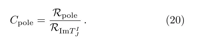
The simple meaning of the correlationCpoleis to answer the following question:When the cut is changed by 100%,how much would the pole location be changed?

To test the correlation between poles and the r.h.c.,we simply setφtest(s)=1.04φ(s),and check the variation of poles and cuts, respectively.The relative uncertainty of the r.h.c.is also estimated by Eq.(19), withsn=(0.1–0.9) GeV2for the isospin-zero S-wave andsn=(0.1–0.8) GeV2for the isospin-one P-wave.The relative uncertainty of the poles and the correlation are calculated in the same way as that of the l.h.c., see Eqs.(19) and (20).

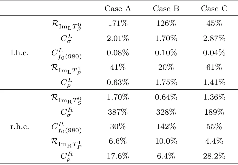
Table 4 The correlation between l.h.c.and poles (represented by superscript‘L’),and between r.h.c.and poles(represented by superscript “R”).

From Table 4, we find thatCRσis roughly two orders larger than that ofCLσ,thoughσis rather close to the l.h.c.Comparing to Ref.[14], which has roughly 15% contribution from l.h.c.,we have a rather smaller contribution from the l.h.c.,caused by the constraint of unitarity on the l.h.c.Also,is roughly three orders larger than that of, andis roughly one order larger than that of.These indicate that the correlation between the unitarity cut and the poles is much larger than that of the l.h.c.and poles.Note that in our case the l.h.c.is not arbitrary but correlated with the r.h.c.,constrained by unitarity and analyticity, see Eq.(11).For each Case,CLσis larger than.This is not surprising as theσis much closer to the l.h.c.Also,CRσis larger than.The reason is that theσis farther away from the real axis, the uncertainty of the pole is larger as the amplitude is continued from the physical region deeper into the complex-splane.It is interesting to see that in averageCLσis roughly two times larger thanAnd for the distance between these poles and l.h.c.(simply sets=0), |sσ| is one half of that of|sρ|, this tells us that the correlation between poles and l.h.c.is inversely proportional to their distance.In contrast,CRσis roughly one order larger than.For the distance between these poles and r.h.c.(simply sets=Respole),|Imsσ|is two times larger than|Imsρ|, this tells us that the correlation between poles and r.h.c.is proportional to their distance.These conclusions are still kept when comparing theσand thef0(980).The discussion of the correlation between poles and cuts reveals that our model, keeping analyticity and unitarity, give strong constrains on poles and l.h.c., even if the pole is a bit faraway from the real axis.

4 Summary

We proposed a dispersive method to calculate the twobody scattering amplitude.It is based on the Omn`es function of the phase, including that of the left hand cut and the right hand cut.The input of the r.h.c.is given by three kinds of parametrizations,and the l.h.c.is solved by Eq.(11), with unitarity and analyticity respected.The pion-pionIJ=00,02,11,20 waves are fitted within our method and the poles and locations are extracted.They are stable except for that of thef2(1270),which lies in the inelastic region.The r.h.c.has much larger contribution to the poles comparing to that of the l.h.c.This method could be useful for the studies of strong interactions in two-body scattering.For instance, it could be applied in theπηscattering, where the correlation between l.h.c.and r.h.c.could help us to constrain the phase shift.Also theππscattering amplitudes obtained here could be used for the future studies when one hasππfinal state interactions, see e.g.Refs.[36–40], and/or to multi-pions, see e.g.Refs.[41–42].

Appendix A:Analytical Amplitudes of Partial Waves Within χPT

The analytical 1-loop amplitudes of these partial waves within of SU(3)χPT are recalculated.For reader’s convenience, they are given below.We have the IJ=00 waves up toO(p4):

Here the superscript ofTin the bracket means the chiral order, and subscripts represent for Isospin and spin, respectively.Note that for reader’s convenience we also give the analytical forms of the imaginary part (r.h.c.) of the amplitudes.TheI=2 S wave is

TheI=1 P wave is

And theI=0 D wave is

It should be noted that in all these partial waves, 2L4+L5and 2L6+L8appear together.[43]TheA,B,Hfunctions are given as below

withρ(t,m)=Notice that our amplitudes are calculated in the formalism ofwhile that of Refs.[44–47]is done in−1.The relation between our LECs (Li) and that of the latter one () is=Li+Γi/32π2.

Acknowledgments

We are grateful to Zhi-Yong Zhou for helpful discussions and for supplying us the files of the SU(2) 2-loopχPT amplitudes.