Stability Analysis of Indirect Adaptive Tracking Systems for Simple Linear Plants with Unknown Control Direction

PAN Qingfei(潘青飞),RUAN Rongyao(阮荣耀),XIE Peng(谢鹏)

( 1.Sanming University,Sanming 365004,China;2.Department of Mathematics,East China Normal University,Shanghai 200241,China;3.School of Mathematics and Statistics,Huazhong University of Science and Technology,Wuhan 430074,China)

Abstract: The paper deals with the adaptive tracker for a class of first-order linear continuous-time plants,with different estimators and modified certainty-equivalence control law.We overcome the difficulty of the loss of stabilizability (or controllability) as the estimate of the plant gain is zero and correct a few substantive mistakes of the results from Middleton and Kokotovic’s paper (1992) about the indirect adaptive regulation of the above-mentioned plant.In the constructed adaptive tracking systems,the explicit expression for the phase-plane trajectories or the explicit solution completely describing the nonlinear behavior of the resultant closed-loop systems is obtained,and some problems of the designed adaptive tracking systems,which due to a loss of stabilizability of the estimated model probably are analyzed.The paper also discusses the impact of these results for the indirect adaptive tracking case of higher order linear continuous-time plants.Meanwhile,we discuss the unknown both control direction and model parameters by making use of the similar pattern.

Key words: Indirect adaptive tracking;Stability analysis;Boundedness property;Control direction;Nonlinear behavior

1.Introduction

Let us consider a plant described by the following model:

whereu(t),y(t) are the plant input and output,respectively,Kpis the gain parameter of the plant,andsdenotes the differential operator.The mimic polynomialsA(s),B(s)are coprime and of degreesn,mrespectively,wherenm,andB(s)is Hurwitz(i.e.B(s)0,∀Res0).

Assume the sign of the plant gain (i.e.the so-called control direction[2−3]of the plant)is unknown in this paper.However,it does usually need to assume that the sign of the plant gain is known both in direct adaptive control and indirect adaptive control[4].In indirect adaptive control,the unknown control direction may cause the loss of stabilizability of the estimated plant model.In particular,the controllability is lost when the estimate of the unknown plant gain is zero.Therefore,the indirect adaptive control with unknown control direction is still a problem which has not been solved completely yet.How to use the different estimators together with a modified certainty-equivalence control law handling the passage of the gain estimate through zero? Which of their signals,if any,go unbounded? Do the causes for unboundedness suggest some“natural fixes”,and should they be in the estimate algorithms or in the control law?

Middleton and Kokotovic[1]answered such basic questions on several extremely simple examples.Unfortunately,it didn’t hit the point.We cite three examples in Section III of [1]as following:

1) For the control law (3.1) (i.e.u(t)=−2y(t)/),if we choose<0 in the case ofb>0,or choose>0 in the case ofb<0,the initial controlu(0)of the resultant adaptive regulation system is positive feedback,which is a mistaken control direction.Its subsequent states will be divergent.Namely,it is impossible for them to keep boundedness properties.Even if sign(b)=1 is known,the control law(3.1)is still incorrect control strategy as selecting the initial estimate<0,which did not completely guarantee the boundedness properties of the controlled states of the resultant closed-loop system.

2) “It is clear from (3.1) that the controlu(t) is grown unboundedly asapproaches zero fory(t)0”.This is a obvious mistake too.Since when→0,althoughy(t)0,it would converge to zero whenconverges to zero,this meansu(t) does not have to be unbounded.Ifu(t) does increase unboundedly,then the boundedness properties of the controlled states of the resultantadaptive regulation system are no guarantee,which denies the main conclusion of themselves.

3)It was a crucial mistake that there is an unstable zero-pole cancellation when dividing the second equation in (3.6) by (3.3),thus the explicit expression of (3.8),the integral curve family defined by the equation(3.7)(see Fig.2 in[1]),is not the phase-diagram of the nonlinear state-space equations (3.2) and (3.3) (since the phase-plane trajectories of this system are undefined at=0),and the boundedness properties ofηsatisfying (3.7) does not mean the boundedness properties ofywhich satisfies (3.2) and (3.3).Therefore the proof of the boundedness properties of the controlled states is incorrect completely.

Even so,[1]is useful in certain sense.It contributes an important result thathas an unchanged sign which characterizes the significant property of related trajectories on the phase-plane.If we can choose sign()=sign(b),which means the sign of the plant gainbneeds to be known,then the boundedness properties could be guaranteed.However,in this case,there no longer exists problem of whetherpasses through zero.For a class of simple linear discrete-time plants,the correspondent adaptive regulation problem had solved completely due to [5].

Enlightened by[1,5],this paper,based on the same simple examples,provides a completely proper answer to the basic question above-mentioned and corrects a few mistakes in[1].We consider the examples of the unstable first-order linear continuous-time plant with the known pole at the right half plane and the unknown both sign and value of the plant gain.Using three different estimate algorithms (i.e.the unnormalized gradient,the normalized gradient and the least squares) and combining with the modified certainty-equivalence pole-placement control law to handle the passage of the plant gain estimate through zero,we proceed on stabilizability analysis by finding the explicit solution to the nonlinear state space equationsor the explicit expression for the phase-plane trajectories,and discuss both boundedness properties and transient behavior of the controlled states of the resultantclosed-loop systems.This analysis provides us with a complete quantitative description of the boundedness properties and their limit properties.

2.The Formation of Adaptive Tracking System

I Plant model

Consider the first-order linear plant

wherey(t)andu(t)are the plant output and input,respectively,andbis an unknown nonzero constant parameter.We assume that an upper bound on the size ofbis known,i.e.

While we assume that the sign ofbis unknown,this is crucial.

Remark 2.1In[1],the lower bound on the size ofbis assumed,that is abs(b)ε>0.But it is only used to SCE control law (2.17) and DCE control law (2.18),not applied to the estimating algorithms(2.6)-(2.9)in[1].In this paper,we don’t need this restricted condition,but we need to know the upper bound of,which may reduce the scope of the selected initial valueso as to move the closed-loop pole to the left plane (e.g.,takes=−1) as soon as possible by adaptive tracking control.

II Parameter estimate algorithms

Assume that the bounded reference signalr(t) is known,which will be the outputy(t)’s tracking target of the resultant closed-loop system.Letb(t) denote the estimate of unknown parameterbat timet.We define the prediction errore(t) of the designed adaptive tracking system is

The regressor in the above case is the scalar (the notation is also applied to the vector case)

Remark 2.2In order to simplify the calculations and avoid the trouble of constructing filters,we assume that the time derivativeof the outputy(t)is available to the parameter estimators.But in order to preserve the realism of the feedback control problem,we also assume that the signalis not available to the feedback control itself.

The following three estimators to be analyzed are standard continuous-time parameter estimate algorithms for updating the parameter estimate[6−8].Each of them defines the rate of changeofb(t)as a function of the regressor,prediction error,and a gain(either a fixedλin the first two cases,or a variablep(t) in the final case).

(a) UG-unnormalized gradient:

(b) NG-normalized gradient:

(c) LS-least squares:

The initial estimate value in the three above algorithms should be selected within[−σ,σ].Without loss of generality,we assume thatλandp(0) are all selected to be positive values larger than 1.

Before we design the feedback control law and proceed with the analysis,let us introduce a property of the LS algorithm established in [1],which effectively eliminates one of the three state components in the analysis (but not in the implementation) of the LS-based adaptive tracking.

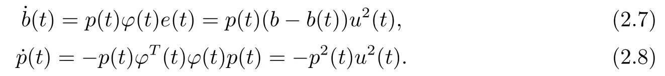
Lemma 2.1For the plant (2.1),the least squares estimators (2.7) and (2.8) have the following property:

Proof of the equality (2.9) had given in Lemma 2.1 of [1].When≠0,the equality(2.10) has deduced immediately from the equality (2.9).

III Control law

Assumption H:The known reference signalr(t) is continuous and bounded,and its time derivativeis also piecewise continuous and bounded.

Leter(t) denote the adaptive tracking error at timet,i.e.,er(t)=y(t)−r(t).We give a modified certainty equivalence pole-placement control strategy,attempting to place the closed-loop pole at the left plane (takes=−1):

whereg(·) is a special sign function,and it is defined as

and

Here the initial timet0may be taken as zero,∆tdenotes a fixed sampling period in the simulations or the implementations of the adaptive tracking control,y(t0) andy(t1) are the outputs of the plant (2.1) at the timest0andt1,respectively,andK(t) are a function about the gainsλorp(t) for the estimators UG,NG or LS.for NG and

The control law (2.11) clearly has a singularity whenb(t) is zero,while it is a removable singularity.Onceb(t) reaches zero at the timet=tz,we can obtain from (2.11) and (2.5),(2.6) or (2.7) that for alln1,t=tz+n∆t,b(t)≡the true valueb(under the cases of used UG,NG or LS estimators) after implementing the control strategyu(er(t),b(t))=1/K(t).

Remark 2.3Although the control direction of the plant (2.1) is unknown,we may guess sign(b)=1.If our guess is really right,the control strategyu(0) defined in (2.11) starts to work whateverb(0) is positive or negative,and can be defined from (2.12) thatg(t)=−1 for alltt0.In this case,the implemented feedback control(2.11)for the plant(2.1)is always negative feedback.If our guess is wrong,then the sign of the plant gainbis negative.It shows that the initial controlu(0) of the adaptive tracking systems is positive feedback,which is a mistaken control direction.It can be calculated from (2.12) thatg(t)=1 for alltt1.Thus subsequent feedback controlu(er(t),b(t)) for alltt1will be corrected immediately as negative feedback.Therefore the control direction ofu(t),∀tt1,defined by (2.11) are always right,and sign(bg(t))=−1,∀tt1.The mistake of the control direction will at the most occur at the timet0,which would not continually affect the succeeding controlled states.

3.Boundedness Properties of the Controlled States

In this section,we now proceed to analyze the three adaptive tracking systems with the modified certainty equivalence pole-placement control law (2.11) and with one estimate algorithm UG,and the rest two trackers (based on the estimate algorithms NG or LS) are omitted,since they follow a similar pattern.An important feature of these analyses is that we generate the explicit expression for the phase-plane trajectories or the explicit solution to the nonlinear state space equations.Therefore,they are able to completely describe the nonlinear behavior of the designed adaptive tracking systems.

Let us analyze the adaptive tracking systems with the unnormalized gradient estimation algorithm UG and the modified certainty equivalence pole-placement control law (2.11).For estimate algorithm UG,formula (2.11) may be rewritten as follows

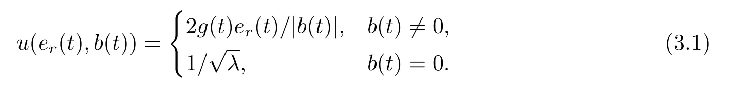
The sign functiong(·) in (3.1) is defined by (2.12).It is clear from (2.11) or (3.1) that the feedback control gain 2g(t)/|b(t)|grow unboundedly asb(t)approaches zero.The sign function in(3.1)is defined by(2.12).It is clear from(2.11)or(3.1)that the feedback control gain grow unboundedly as approaches zero.The main question here is that whether such an unbounded feedbackcontrol gain will force the controlled state of the designed adaptive tracking system to grow unboundedly.Our answer is in the negative for such adaptive tracking system.Even whenb(t) passes through zero,the controlled states remain bounded and their transients are well behaved.

In this case,the state vector of the designed adaptive tracking system is composed of both the tracking errorer(t) of the resultant closed-loop system and the estimateb(t) of the plant gainb.For convenience of both analysis and simulation,the true value of the plant gainb,unknown to the designer,is assumed to be

or

The other assumption for simplification of calculations is that the time derivativeof the tracking errorer(t) is available to the parameter estimator,otherwise,the two filters will be introduced like what was done in [9-10].To preserve the realism of the feedback control problem,we also assume that the signalis not available to the feedback control itself.

Using (2.1),(2.3)-(2.5),(3.1) ander(t)=y(t)−r(t),we can write the nonlinear statespace equations as

In the above (3.5),the true value is given by (3.2).If the true value isb=−1 given by(3.3),then the estimate formula (3.5) ofbshould be replaced by

It is easily observed thater(t)≡0 is an equilibrium manifold of (3.4) and (3.5) or is also the one of (3.4) and (3.6),and that the equilibria inside the segmentsb(t)∈[0,2]orb(t)∈[−2,0]are stable,while those outside segments are unstable.Possibly there exist two kinds of tendency of trajectories for the unstable cases:tend to an equilibrium or depart from all the equilibria.

It is clear from(3.5)thatb(0)=1 impliesb(t)=1 for allt0.Henceb(t)≡1(∀t0)is an invariant manifold of the differential equations(3.4)and(3.5),and its equilibrium solution under the initial condition ofb(0)=−1 is

It is also clear from (3.6) thatb(0)=−1 impliesb(t)=−1 for allt0.Henceb(t)≡−1(∀t0) is also an invariant manifold of the differential equations (3.4) and (3.6),and its equilibrium solution of (3.4) and (3.6) under the initial condition ofb(0)=−1 is

These mean that ift=0,the estimateb(0) is correct,i.e.it equals the true valueb=1 orb=−1,then b(t) will continue to be correct for allt0.

The two invariant manifold pairs{er(t)≡0,b(t)≡1} and{er(t)≡0,b(t)≡−1} of the two designed adaptive tracking systems divide respectively the corresponding phase-plane into four invariant quadrants.Further insight into the shape of the phase trajectories within each quadrant is provided by the fact thatb(t) defined by (3.5) or (3.6),respectively,is all of constantsign,i.e.

or

Thus,we know respectively from(3.9)and(3.10)thatb(t)is monotonically decreasing forb(0)>1,orb(0)>−1,and monotonically increasing forb(0)<1,orb(0)<−1.No matter what sign of the plant gainbis positive or negative,the equation (3.4) can be rewritten as follows

wheret1is given in (2.13).Ifer(0)≠0,we find the solution of (3.11) as

where

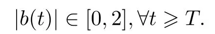
If abs(b(0))∈(0,2),then abs(b(t))∈(0,2),∀t0.It infers from (3.13) thatf(t1,t) ≤0,∀tt1Hence the explicit solutioner(t) of (3.11) is of boundedness property,and furthermore

This implies that under the condition of|b(t)|∈(0,2),∀t0,|b(t)|is strictly decreasing and so it is of limit zero,i.e.limt→∞er(t)=0.Therefore the differential equations (3.4),(3.5)and (3.4),(3.6) are all asymptotically stable.

If|b(0)|=2,then both=0 and=0.This shows that they are critical points of the above-mentioned differential equations.Furthermore,bother(t) andb(t) are bounded.Also,the boundedness property ofy(t) is deduced from Assumption H about reference signalr(t) ander(t)=y(t)−r(t).

Remark 3.1For the above-mentioned adaptive tracking system,we require|b(0)|∈[0,2]to ensure the boundedness properties and the convergency of{er(t),y(t),b(t);∀t0}.This is a sufficient condition but not necessary.In fact,simulation examples in next section show that the designed adaptive tracking systems are asymptotically stable and the controlled states are bounded even if|b(0)|>2.Also there exists a finite timeT0 such that

Meanwhile,we also have

In particular,if the true value is given by (3.2) or (3.3),andb(0) is selected asb(0)=−4 orb(0)=4,for the above three parameter estimate algorithms,then they can makeb(t) pass through zero without destroying the stability of the designed adaptive tracking systems.Also,two simulation examples in next section show that Assumption H about the time derivative ˙r(t) of the reference signalr(t)( i.e.it is piecewise continuous and bounded) is needless too.

4.Simulations of Adaptive Tracking Systems

In Section 3,boundedness properties and convergency of the controlled states for the resultant adaptive tracking systems have been analyzed,which are mainly involved with limit property.Two simulation examples in this section are given to show the performance of the resultant adaptive tracking systems on the finite time zone.

Example 4.1Simulation of adaptive tracking control for the plant (2.1) under the assumption (3.2) and two groups of suitable initial values.

First,we use the control law (3.1) with the update law (2.5) for the adaptive tracking simulation of the plant (2.1).In this example,tracked target of adaptive tracking control is the sinusoidal signal

Select the UG-estimating gainsλ1=180 andλ2=192 for two different groups of initial value{y1(0)=e1r(0)=0.06,b1(0)=4} and{y2(0)=e2r(0)=−0.06,b2(0)=−4}.Here we proceed to simulate,namely find digital solutions of the nonlinear differential equations (3.4)and (3.5) with some initial conditions chosen above.The simulation results are given in Fig.4.1-4.4.

In Fig.4.1,the outputs arey1(t) andy2(t) for the corresponding{λ1,y1(0),e1r(0),b1(0)}and{λ2,y2(0),e2r(0),b2(0)},respectively,wherey1(t)−0.4 andy2(t)+0.4 denote the curvesy1(t)andy2(t)downwards and upwards to move 0.4 unit altitude respectively.u1(t)andu2(t)in Fig.4.2 denote the control quantities,respectively,corresponding to the two groups of the initial values.In Fig.4.3,the adaptive tracking errorseir(t)(i=1,2) also correspond to the two groups of the initial values,respectively.In Fig.4.4,b1(t) andb2(t) are the curves of the estimate values of the plant gain,respectively,corresponding to the two groups of the initial values.In simulation,we set a fixed sampling period ∆t=0.004 seconds for the sampledcontrol system and the movement time 80 seconds for trajectories,but only 16 seconds picture is drawn in Fig.4.4 because the parameter estimators are convergent so fast.

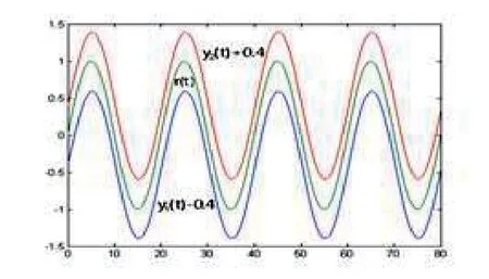
Fig.4.1 Outputs yi(t)(i=1,2) tracking r(t)=sin(0.01πt) defined in (4.1)

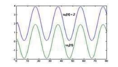
Fig.4.2 Control quantities ui(t)(i=1,2)versus time t

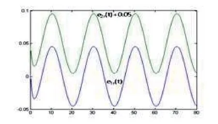
Fig.4.3 Adaptive tracking errors eir(t)(i=1,2) versus time t

Fig.4.4 UG-estimates bi(t)(i=,1,2) of the plant gain b versus time t

Example 4.2Simulation of adaptive tracking control for the plant (2.1) under the assumption (3.3) and two groups of suitable initial values.

The adaptive tracking reference signalr(t)=sin(0,01πt) in Example 4.1 is replaced to the following rectangular wave:

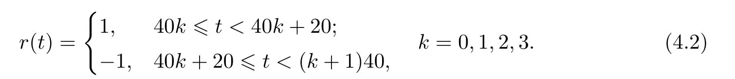
The functionr(t) is piecewise smooth and its derivative is the sum of four pairs of positive and negative impulse functions,i.e.,

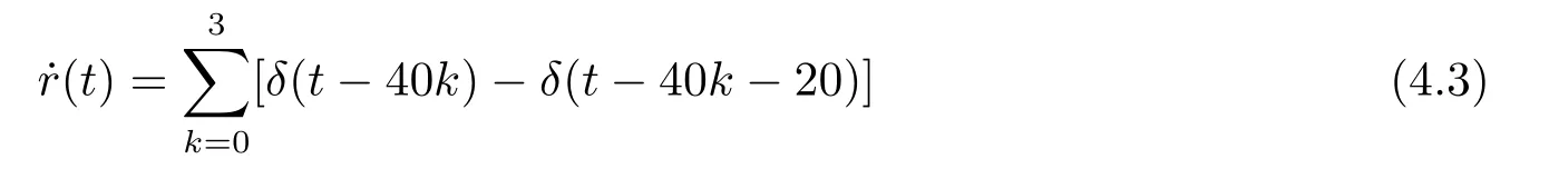
In this case,the equation (3.4) is unchanged and the equation (3.5) is replaced by the equation (3.6).We still use the control law (3.1) with the update law (2.5) for the adaptive tracking simulation of the plant(2.1).Two the UG-estimating gainsλi(i=1,2)and different group of initial values are selected the same as Example 4.1.The simulation results are given in Fig.4.5-4.8.

Fig.4.5 Outputs yi(t)(i=1,2) tracking r(t) defined in (4.2)

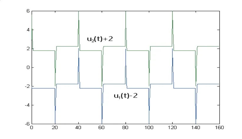
Fig.4.6 Control quantities ui(t)(i=1,2)versus time t

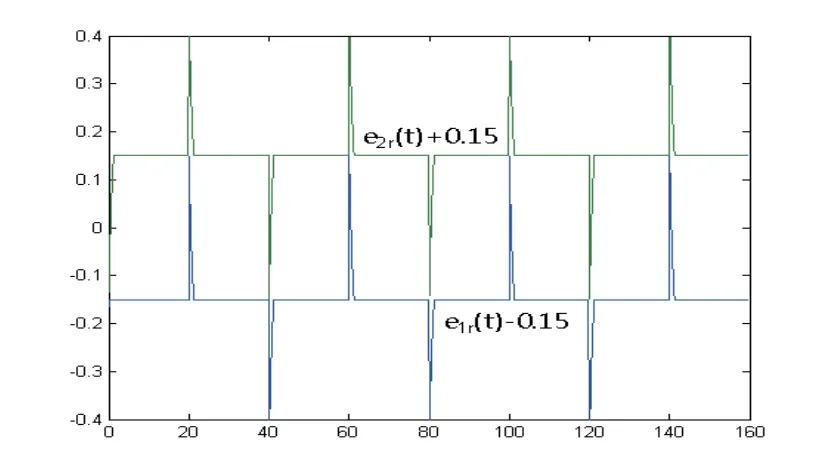
Fig.4.7 Adaptive tracking errors eir(t)(i=1,2) versus time t

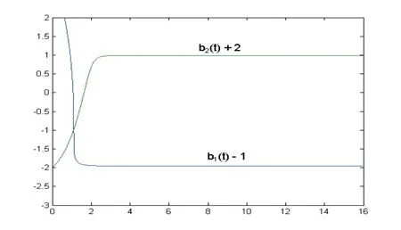
Fig.4.8 UG-estimates bi(t)(i=1,2) of the plant gain b versus time t

We also use the control law(2.11)with the update estimate(2.1)or(2.7)for the adaptive tracking simulations of the plant(2.1).The simulation results are similar to the corresponding results of the UG-based adaptive tracking simulation.Therefore we omitted their simulation pictures.It should be noted when the simulation is going on with the LS estimate algorithm,and initial valuep(0)should be selected much larger than the values of two parameter estimate gainsλ1andλ2.Otherwise,the excitation signal could be too weak hard to guarantee the convergence rate of the parameter estimateb(t).

5.Conclusions

Under the conditions of unknown both sign and value of the plant gain,although the sign of the initial estimates of the plant gainbi(0)(i=1,2) are probably incorrect,the three parameter estimate algorithms respectively combining the modified certainty equivalence control law are all able to drive that the estimatorsb(t) pass through zero and quickly converge to the true value ofb.Thus,the controlled states of the designed adaptive tracking system are bounded,and the tracking errorser(t)→0(t→∞).At the same time,their transients are well behaved.

For the higher order plant (1.1) with the unknown control direction,we can generalize the modified certainty-equivalence control strategy (2.11) to the plant (1.1),and attempt to place all the closed-loop poles ats=−1.Under this case,b(t) in the control strategy (2.11)is replaced byKp(t).We can still use three estimate algorithms UG,NG and LS to estimateKpand all the unknown parameters of bothA(s) andB(s) in (1.1).The indirect adaptive control problem with unknown control direction can be solved as long as we select properly the estimate gainλfor UG and NG,in particular,select carefully the initial valuep(0) of the estimate gain for LS.