On developing data-driven turbulence model for DG solution of RANS

Ling SUN, Wei AN, Xuejun LIU,c,*, Hongqing LYU

a College of Computer Science and Technology, Nanjing University of Aeronautics and Astronautics, Nanjing 211106, China

b College of Aerospace Engineering, Nanjing University of Aeronautics and Astronautics, Nanjing 210016, China

c Collaborative Innovation Center of Novel Software Technology and Industrialization, Nanjing 210093, China

KEYWORDS

Abstract High-order Discontinuous Galerkin (DG) methods have been receiving more and more attentions in the area of Computational Fluid Dynamics (CFD) because of their high-accuracy property.However,it is still a challenge to obtain converged solution rapidly when solving the Reynolds Averaged Navier-Stokes(RANS)equations since the turbulence models significantly increase the nonlinearity of discretization system.The overall goal of this research is to develop an Artificial Neural Networks (ANNs) model with low complexity acting as an algebraic turbulence model to estimate the turbulence eddy viscosity for RANS. The ANN turbulence model is off-line trained using the training data generated by the widely used Spalart-Allmaras (SA) turbulence model before the Optimal Brain Surgeon(OBS)is employed to determine the relevancy of input features.Using the selected relevant features,a fully connected ANN model is constructed.The performance of the developed ANN model is numerically tested in the framework of DG for RANS, where the‘‘DG+ANN” method provides robust and steady convergence compared to the ‘‘DG+SA”method. The results demonstrate the promising potential to develop a general turbulence model based on artificial intelligence in the future given the training data covering a large rang of flow conditions.

1. Introduction

Numerical simulation of turbulent flows remains an ongoing challenge in computational fluid dynamics due to computational requirements, multiple time scales and difficulties involved in modeling. The Direct Numerical Simulation(DNS)1can obtain accurate information of the turbulent flow field and is an effective method to study the turbulence mechanism.However,existing computational resources often struggle to meet the needs for high Reynolds number flow simulations, which limits its application in engineering.Large-Eddy Simulation (LES)2requires less computational resources since it only resolves large energy-carrying scales of motion and models the sub-grid unresolved scales. However,it is also far away from solving complex engineering problems.A popular alternative is to solve the Reynolds Average Navier-Stokes(RANS)equations3which requires less computational costs compared to the direct numerical simulation and the large-eddy simulation but needs turbulence models to ensure the closure of the equations.

Previous studies have shown that machine learning seems a promising technique to release the obstacles in RANS simulation. There have been some interesting attempts of using machine learning methods to model turbulence. Tracey et al.4applied a new machine learning algorithm which extended kernel regression to improve low-fidelity models of turbulence,and combustion and obtained error bounds.Milani et al.5used a random forest model to determine the turbulent diffusivity in film cooling flows and showed significant qualitative and quantitative improvement over the usual turbulent Prandtl number.Tracey et al.6developed the functional form of a turbulence model by applying machine learning techniques and demonstrated that a trained neural network reproduced the Spalart-Allmaras (SA) model in a wide variety of flow conditions from 2-D flat plate boundary layers to 3-D transonic wings. Zhang et al.7evaluated different machine algorithms including Gaussian process regression and Artificial Neural Networks (ANNs) to reconstruct the function forms of spatially distributed quantities extracted from high fidelity simulation and experimental data.Ling et al.8utilized three classifiers including a support vector machines, an AdaBoost decision trees and a random forest to identify regions where RANS simulation yields uncertain results. Chang et al.9proposed two data-driven methods which were Common-grid POD and Kernel-smoothed Proper Orthogonal Decomposition(POD) to predict flow fields. The experiment demonstrated that the model successfully reproduced the LES model and the turnaround time for predicting a new design point was 2000 times shorter than the LES simulation. Deep neural networks and random forest regression were used to predict the wall pressure fluctuation power spectrum using the no-local and local variables10. The study significantly obtained more satisfactory results compared with deep neural networks barely using local variables11. Karthikeyan et al.12used the machine learning to reconstruct the functional forms by applying inverse problems to computational and experimental data.Although the studies mentioned above are still in an early phase, many authors consider that machine learning algorithms as a potential way to improve the flow field analysis.

Previous works have shown that multi-layer feedforward neural network has the ability to identify and reproduce the highly nonlinear behavior of the turbulent flows13.Proofs have also shown that Artificial Neural Networks (ANNs) can be used, with satisfactory results, as curve fitting and modeling techniques to discover the relationships among different variables14-16. The work in Ref.13computed the turbulent viscosity coefficient using information of both the derivatives of instantaneous velocities of the turbulent flux and the Reynolds tensor components.All the above-mentioned attempts indicate that the machine learning methods are beneficial to analyzing the turbulence. However, the performance of the data-driven turbulence models in the high-order Discontinuous Galerkin(DG) solution of RANS has not been investigated.

It has been found that the efficiency and robustness of the convergence are significantly reduced since the widely used turbulence models (one equation model or two equation models)increase the complexity of the numerical discrete system, particularly when high-order numerical schemes (such as the DG17methods) are employed18, for which further improvement on the turbulence model for RANS is expected. In this paper, an ANN turbulence model is developed to simplify the DG discrete system of RANS and improve the efficiency and the robustness of the convergence, which is generated based on the training data from the RANS with SA model19.The structure of the ANN model is optimized using the Optimal Brain Surgeon(OBS)20,21for examining the contributions of input variables and setting a criterion to select relevant features.

The remaining of this paper is organized as follows.Section 2 explains the adopted machine learning approaches including the artificial neural networks and the optimal brain surgeon. Section 3 describes the problem formulation and the DG solution framework used here. Section 4 details the configuration of the developed methods. The simulations and discussion are given in Section 5. Finally, we conclude in Section 6.

2. Machine learning methodology

2.1. Multi-layer perceptron

A Multi-Layer Perceptron (MLP) is a feedforward artificial neural network model22where a large number of processing nodes are interconnected in a directed acyclic graph to map from input data space to output space. The processing node is the simplest unit of the calculation that takes a weighted sum as input, sends the weighted sum, bk, to an activation function and outputs the result, yk(see Fig. 1).

Fig. 2 shows a schematic of a basic multi-layer perceptron used in this study. In this architecture, the net begins with the feature vector,x,which is used as the input to the first hidden layer. This process is repeated until the output node is reached. For this sample architecture, the value of the hidden layers (z1，1，z1，2，...，z1，H1) are constructed as23:

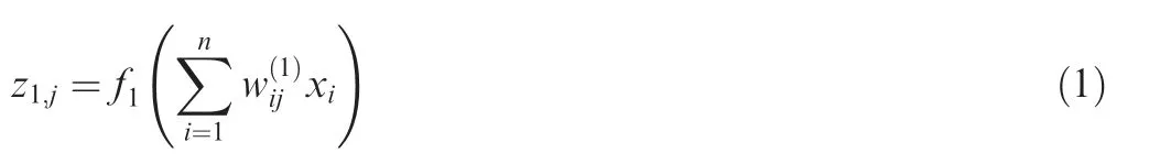
where f1and wij(1)are the activation function and the weight,respectively, associated with the connection between xiand node j in the first hidden layer. Similarly, the second hidden layer nodes are constructed as:

Fig. 1 A processing unit of MLP.

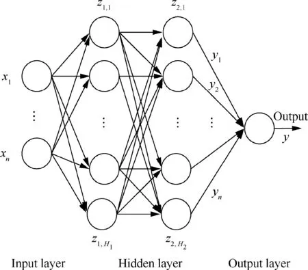
Fig. 2 Schematic of MLP.

Finally, the output node is

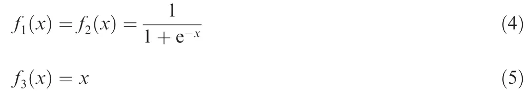
Except the input layer nodes, all nodes in the other layers contain either linear or non-linear activation functions.In general, when the MLP is used for function approximation, f1, f2are non-linear and f3is linear. For example, the formulation adopted for f1, f2and f3can be as follows:

The weight values w(1),(2),(3)are the free parameters of the MLP which need to be estimated byoptimizing‘loss function’:

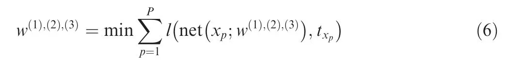
where net(xi;w(1),(2),(3)) is the predicted value at data xiand is calculated by the MLP given the weights w(1)(2)(3),txiis the corresponding true output value, P denotes the number of training data, and l is the loss function. The BackPropagation(BP) algorithm is the most popular technique for multi-layer neural networks to obtain weight gradients and the gradientbased optimization algorithms are used to estimate the optional values of weights24.

2.2. Optimal brain surgeon

Optimal brain surgeon belongs to a class of post training pruning algorithms25for multi-layer perceptrons. The algorithm normally begins from the trained neural network which has adequate performance. The pruning process seeks to prune any network parameter including the individual weights and the input units that have the least increase in the training error according to the information in the second-order derivatives of the error surface.

In general,we seek to optimize the following error function through training the multi-layer perceptron:

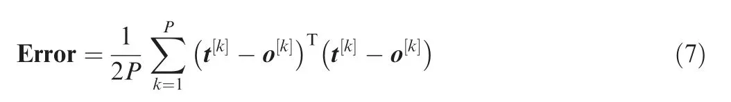
where Error is the error, t[k]and o[k]are the desired response and network response for the kth training data, respectively.

The functional Taylor series of Error with respect to the weights is20:

where H is the Hessian matrix.As long as the network training converges to local minimum,the first term will vanish to zero.In our work we also ignore the third and all higher order terms. Our goal is then to set one of the weights (which we denote wz) to zero to optimize the increase in the error given by Eq. (7). The optimization goal is set as:

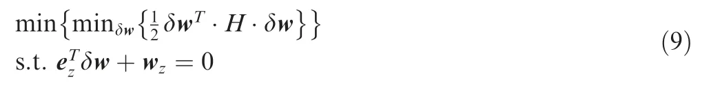
where ezis the unit vector in the weight space corresponding to weight wz.

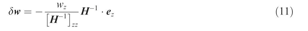
For this optimization problem,we form a Lagrangian given by:

where λ is a undetermined Lagrange multiplier. The optimal change in weight is

The resulting change in training error Lz,which also shows the sensitivity of weight z, is

In this study,we evaluate Lzto determine the sensitivity for each weight to the output variable and select the most relevant input features by summing the sensitivity of all related weights.

3. Embedding ANN in turbulence model

3.1. DG solution of RANS

Since DNS and LES are still expensive for complex problems,RANS still plays an important role in engineering, which is generated from the original N-S equations through averaging procedures26. Various turbulence models are introduced to close the RANS equations. The SA turbulence model is a widely used one.

The RANS equations with the SA turbulence model can be reformulated as:

where

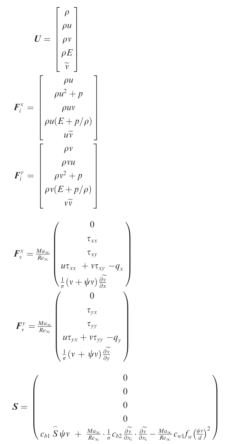
The 5th equation in Eq. (14) is the SA model18,26, which is also called one-equation turbulence model introduced to finish the turbulence closure. There are some two-equation turbulence models,which introduce two more equations to the original Navier-Stokes equations26. The simplest way to compute the eddy viscosity is the zero-equation models, which are also denoted as algebraic models, for which the eddy viscosity is calculated directly from some local flow conditions and the 5th equation in Eq.(14)does not exist.Although the algebraic models are much cheaper for computation,the accuracy of the algebraic models is normally not comparable with those oneequation and two-equation models.26

By choosing suitable shape functions φjand appropriated numerical solutions Uhat each cell e, we obtain the weak formulations of Eq. (13):

where Ω，e and σ are the domain and the boundary of cell e.n is the normal vector to the boundary pointing outward. The well-known local Lax-Friedrichs flux function for the approximate solution of Riemann problem is used to define inviscid numerical flux FiUh( )·n. As for the viscous numerical flux FνUh，Θ( )·n,BR-2 scheme is used.More details of the DG discretization can be found in Ref.18.

The DG discretized equations Eq.(15)leads to a system of nonlinear ordinary differential equations which can be rewritten as:

where M is the mass matrix arising from discretization of the first term of Eq. (16) and R(u) the residual vector. With the backward Euler difference method,the following linear system is obtained:

where Δu=un+1-unand A = M/Δt+∂R/∂u

(). Considering that matrix A is always a large sparse block matrix, GMRES method is used to solve the linear system.

Fig. 3 Procedure of generating the ANN turbulence model.

Fig. 4 Mesh generated by DG solution.

Fig. 5 Mach number contours computed with different orders.

The equation of the SA model in RANS equations increases the complexity of the final discrete system, which reduces the robustness of the convergence of the DG solution18.If the SA turbulence model is replaced by algebraic turbulence models,the final discrete system can be significantly simplified. The main problem is that the traditional algebraic models are normally not as accurate as the SA model.In order to improve the accuracy and the efficiency of the DG solution of RANS,a data-driven algebraic turbulence model is going to be developed based on artificial neural networks in the following sections.

Fig. 6 Turbulence eddy viscosity with different orders.

3.2. Solution framework

Fig.3 shows the procedure of generating the ANN turbulence model used in this work.In this framework the machine learning model based on the training data is created.First,the training data is generated by solving the RANS with the SA model using the DG method. Second, the gradient-based algorithm(Levenberg-Marquardt algorithm in this work) is employed to train the ANN based on the training data, where cross validation is used to select the optimal structure of the network.Third, in order to determine the relevant input variables to eddy viscosity we propose the use of OBS strategy for identifying the most pertinent flow-field features and network pruning.In addition, the proposed technique is compared to the stateof-the-art feature selection algorithms including TreeBagger27and ReliefF28,for the validation of the selected important features. Next, the ANN model is trained once again using the selected features.Finally,the optimized ANN model is applied as the surrogate model instead of the complex SA model, and performs as the algebraic models in CFD. By testing the obtained ANN model with new cases, the performance of the new model can be evaluated.If the accuracy is not satisfied,a re-sample process can be launched to generate more data covering a larger range of flow conditions.Then another cycle of model construction follows.The whole procedure continues until acceptable results are achieved.In the following sections,we will use the simulations from a range of flow conditions to show the usefulness of the proposed method in stabilizing the DG solutions of RANS.

4. Numerical setup

4.1. Configuration

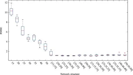
Fig. 7 RMSE for various network structures.

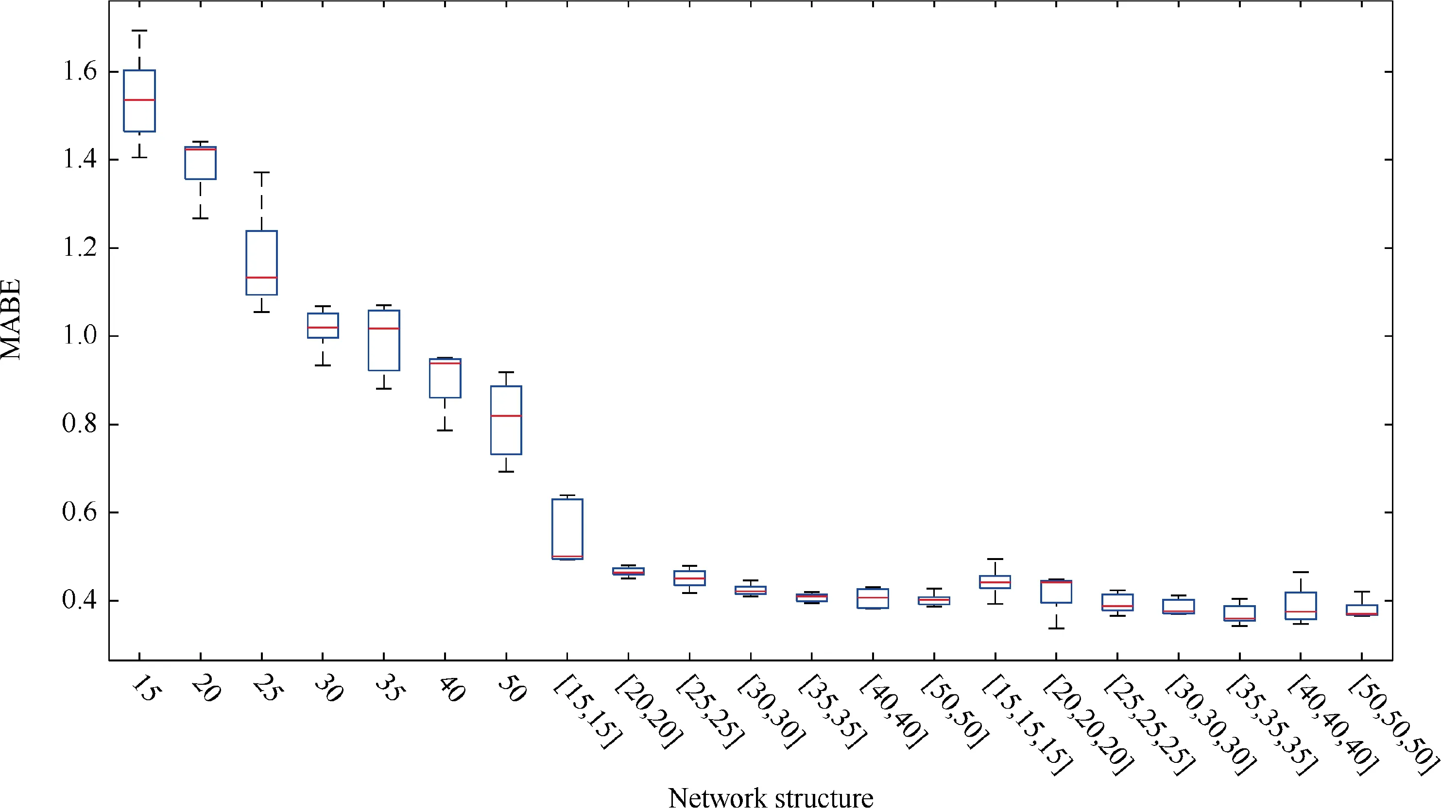
Fig. 8 MABE for various network structures.

4.2. Generation of the training data

The training data used in this paper is generated by solving the RANS with the DG method described in Section 3.Instead of using a large number of grid elements, the accuracy of DG methods can also be improved by increasing the order. In this section,the accuracy of the DG solution of the RANS with SA turbulence model is numerically tested.

Fig. 4 displays the used mesh of the NACA0012 airfoil which contains 2576 elements.The Mach contours and the turbulence eddy viscosity computed with different orders(p=0,1,2,3) for the case of Ma=0.3 are given in Figs. 5 and 6, where the accuracy of the DG solution is improved when the order p is increased from 0 to 2. The color scale one the right in each plot indicates the value of the eddy viscosity coefficient. The p2 solution and the p3 solution agree very well and no significant difference can be observed which means the p2 and p3 DG solutions on the mesh in Fig.4 are accurate enough and the accuracy of the DG solution can not be further improved by increasing the order of DG. Then the p3 DG solutions on the mesh in Fig.4 will be used as the training data in this paper.

4.3. Network setup

Before training the ANN model, the data are normalized.There are a variety of practical reasons why standardizing the inputs can make training faster and reduce the chances of getting stuck in local optima. In addition, weight decay and Bayesian estimation can be done more conveniently with standardized inputs. We also aim to seek the underlying mappings from the input features to the eddy viscosity under any cases. For these reasons, the inputs from all cases are pooled together and scaled in range [-1,1] in this study.

In regression problems, the activation function of the hidden neuron is normally chosen to be non-linear, for example,the sigmoid function and the Rectified Linear Unit (ReLU)function. In this study, the sigmoid function in Eq. (4) and the linear function in Eq. (5) are used for hidden and output neurons, respectively.

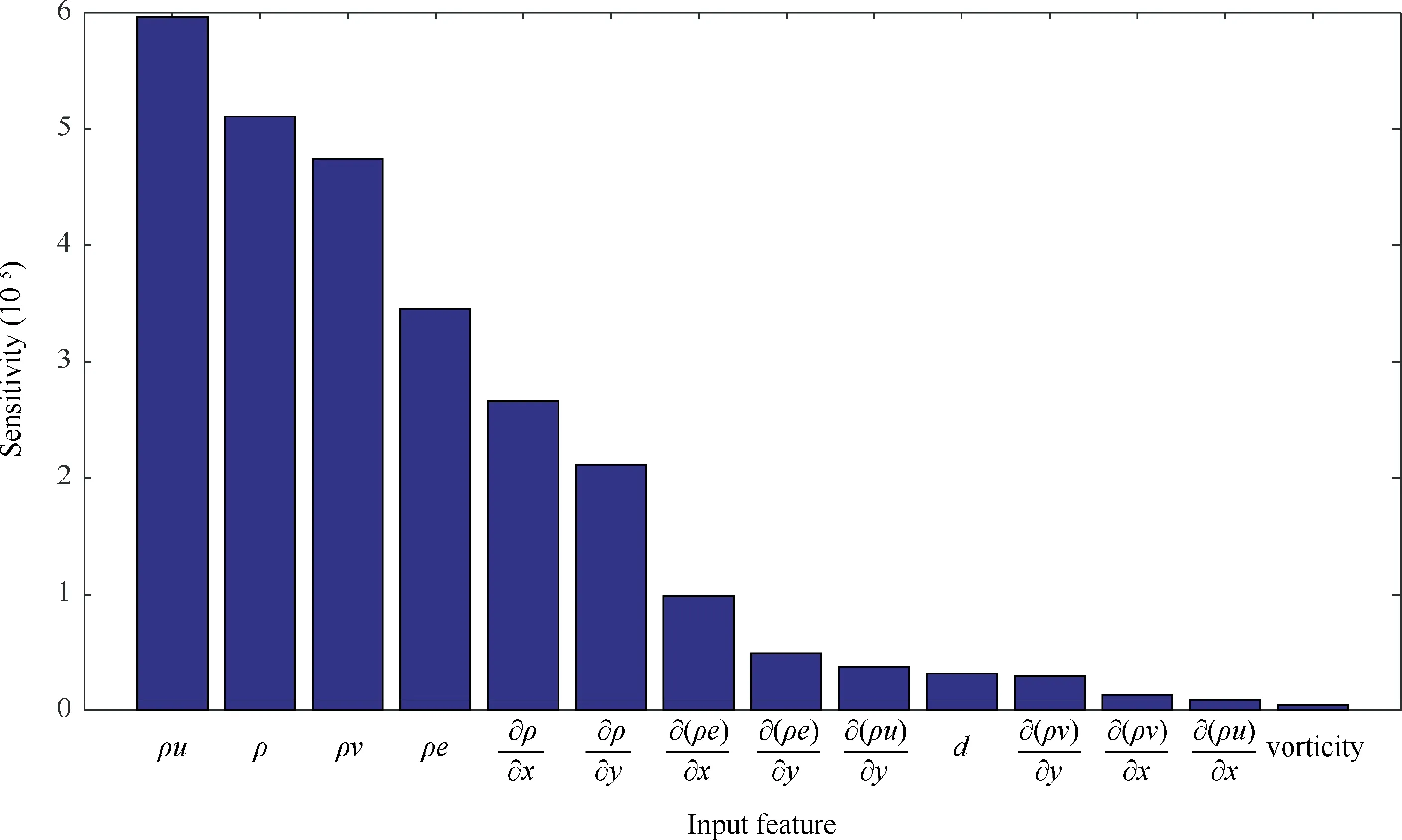
Fig. 9 Sensitivity of input features in MLP-OBS strategy.

Fig. 10 Feature importance calculated from ReliefF algorithm.

In machine learning, the vanishing gradient problem is a difficulty found in training ANN with backpropagation. In order to avoid the occurrence of gradient explosion and gradient vanishing,the number of hidden layers is normally set less than four.We therefore investigate network structures with up to three hidden layers by evaluating the prediction accuracy of the networks. Besides, parameters including weights and thresholds are initialized in range [-1,1]. The gradient-based algorithms, Levenberg-Marquardt algorithm, for weight estimation is adopted in this work,and an early stopping strategy is used to effectively avoid over-fitting.

Fig. 11 Feature importance calculated from TreeBagger.

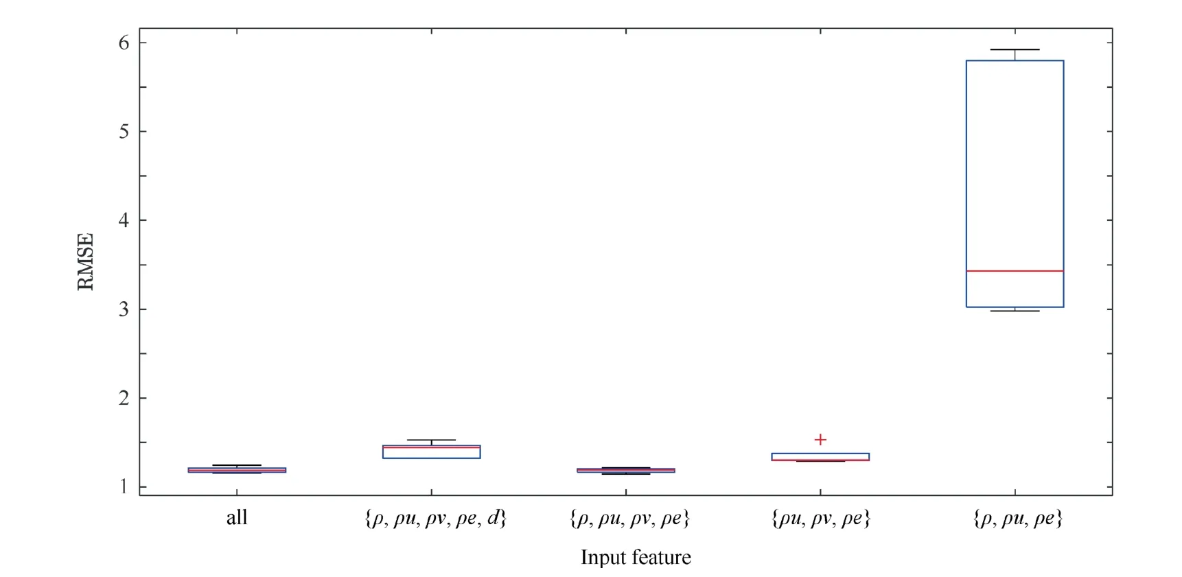
Fig. 12 Validation of feature selection calculated from 10 runs of ANN.

Fig. 13 Zoomed-in version of the first three combinations in Fig. 12.

5. Simulation and discussion

5.1. Evaluation of performance of models

Several quantities are used to measure the accuracy of the ANN model. In this study, the model prediction results are validated in terms of Root-Mean-Square Error (RMSE)and Mean-Absolute Bias Error (MABE) which are defined as:where y and ypare the true and predicted values, respectively,and N is the number of the test data.

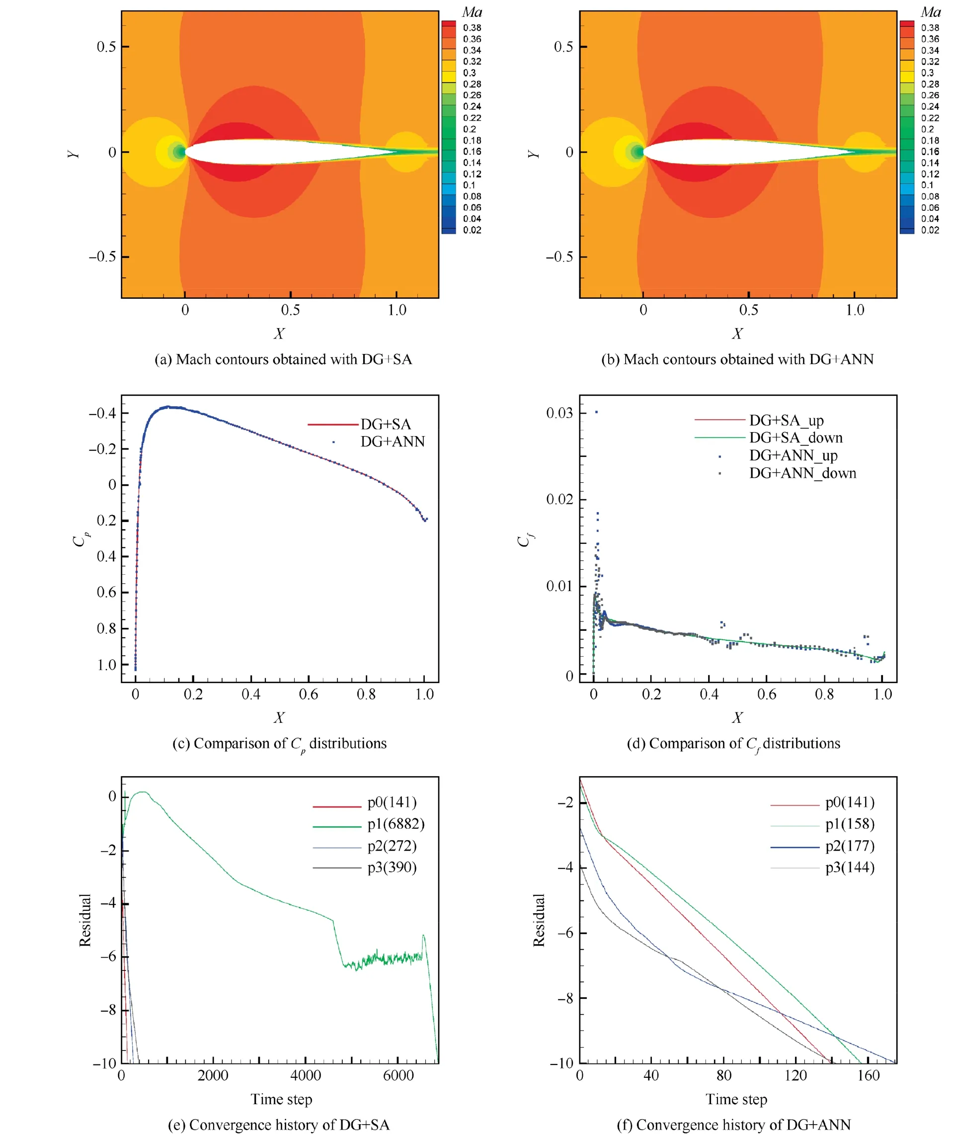
Fig. 14 Comparisons of the performances of the DG+SA and DG+ANN (Case-1).

5.2. Selection of structure of neural networks

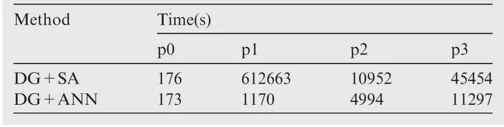
Table 1 Time consuming of DG+SA method and DG+ANN method (Case-1).

Fig. 15 Comparisons of the performances of the DG+SA and DG+ANN (Case-2).

Comparative analysis of the different structures of fully connected neural network are conducted in this section. In our experiment, the number of hidden layers in fully connected neural networks varies among 1, 2 and 3. RMSE and MABE are estimated on test data sets for the evaluation of the prediction accuracy of various networks.Each neural network structure runs for 10 times to avoid the effects of the randomness of weight initialization.We use 70%of data for training,15%for validation and 15% for testing. Figs. 7 and 8 demonstrate the RMSE and MAPE boxplots, respectively, for all 21 network structures with the number of neurons for each hidden layer shown on X-axis. As the number of hidden neurons increases,the test error decreases gradually. It is obvious that among all the fully connected neural networks,the error of test data sets is relatively stable after the neural networks with two hidden layers. The neural networks with only one hidden layer performs obviously worse than the two-layer networks showing the disability to capture the non-linear relationship between the input and eddy viscosity.Conversely,it does not mean that networks with too deep structures certainly perform well due to the difficulties involved in optimization with many local minima. Therefore, we choose two hidden layers for the further experiments with OBS. In fact, it has been shown that the two-layer neural network has the capability to approximate any measurable function to any high accuracy.29

Fig. 16 Comparisons of the performances of the DG+SA and DG+ANN (Case-3).

Table 2 Time consuming of DG+SA method and DG+ANN method (Case-2).

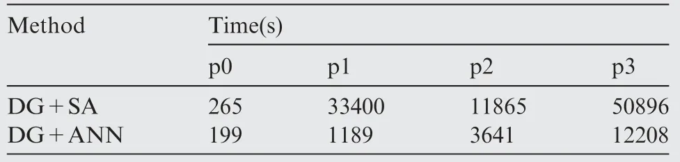
Table 3 Time consuming of DG+SA method and DG+ANN method (Case-3).

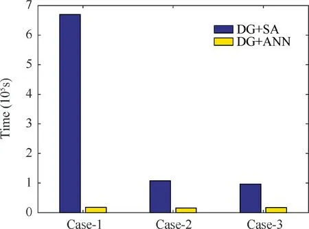
Fig. 17 Comparisons of the total CPU time to obtain p3 DG solution.

5.3. Sensitivity analysis

The relative contribution of each input feature in estimating eddy viscosity is assessed by sensitivity analysis. Hussain et al. applied OBS strategy to select relevant input features of the neural network in the modelling of solar radiation.30Hussain assumed that the contribution of input variables to the output variable was equal to the number of connections between the input layer and the first hidden layer. However,this strategy ignores the strength of the individual connection.Note that input variables with the same number of connections can have unequivalent contribution to the prediction of the output variable for the reason that different values of weights can be associated with these connections. Therefore, this approach can’t fairly evaluate the relevance of input features with the output variable. In this paper, the sensitivity of an input feature is obtained by summing the sensitivity of weights calculated by Eq. (12). It therefore considers both the number of connections and connection strength. Fig. 9 shows the ordered sensitivity of input features produced by our MLPOBS strategy.Overall,ρ，ρu，ρv and ρe have high contributions as compared to other variables. Since the other features show less sensitivity to the target,they can be eliminated in order to simplify the network structure and achieve higher prediction accuracy.

The proposed strategy to determine importance of input features is compared with the other two state-of-the-art feature selection algorithms, ReliefF27and TreeBagger28. ReliefF is a unique family of filter-style feature selection algorithm that can be capable of correctly estimating the quality of attributes in regression problems with strong dependencies between features. Fig. 10 shows the feature importance calculated from ReliefF algorithm.Positive feature importance indicates a positive correlation with eddy viscosity, otherwise the negative feature importance are redundant to estimate eddy viscosity.It can be seen from Fig. 10 that the features including ρ，ρu，ρv，ρe, and d are most relevant to the target. Obviously,the ρu shows the strongest importance to eddy viscosity.These results are consistent with those found by our MLP-OBS approach.

The decision tree algorithm is also used to select relevant features. Since an individual tree tends to be overfitting,TreeBagger algorithm combines the results of multiple decision trees, and thus reduces the effect of overfitting and improves the generalization. Fig. 11 demonstrates the results of TreeBagger which lead to the similar conclusion that ρ，ρu，ρv，ρe and d have relatively large contributions compared to other features.

From the above results of all the three feature selection methods,we find that the ρ，ρu，ρv，ρe have the most significant effects on the prediction of eddy viscosity from all the three feature selection methods. It is therefore possible to construct a simplified neural network that has improved performance using the selected most important features.

Fig.12 demonstrates the RMSE boxplots of different combinations of important features. For better visualization,Fig.13 shows the zoomed-in version of the first three combinations in Fig. 12. It can be seen from Figs. 12 and 13 that the neural network achieves the highest accuracy and the algorithm becomes stable by using the combinations of the four most important features,ρ，ρu，ρv and ρe.When using five features by adding d, the capability to estimate eddy viscosity becomes unstable and the RMSE increases.On the other hand,eliminating any of the four features will bring rapid increase in the prediction errors. We therefore consider that these four features are indispensable in order to obtain high prediction accuracy.

5.4. Description of the eddy viscosity

We obtain the parameters when the neural network is trained.The detailed description of eddy viscosity calculated from the machine learning are constructed as:

where f1and X are the activation function and input, respectively.Wiand Biare the weight and bias in layer i respectively.Out is output of neural network.

Finally the eddy viscosity is anti-normalization:

where vis is the eddy viscosity, ymaxis the maximum value of the eddy viscosity in training data.

5.5. Behavior of the proposed ANN model

In order to test the accuracy of neural network, we first attempt to embed the neural network into the RANS equations. The neural network is off-line trained using the training data set obtained from the ‘‘DG+SA” simulations at flow conditions of Ma=0.3, 0.31, 0.32, 0.33, 0.34, 0.35, α=0°and Re=1850000. The obtained ANN turbulence model is then used as an algebraic turbulence model and the RANS is solved with DG in three cases different from the training cases:Case-1 (Ma=0.335, α=0°, Re=1850000), Case-2(Ma=0.28, α=0°, Re=1850000), Case-3 (Ma=0.3,α=2.0°, Re=1850000). In order to ensure the convergence,the p order simulations starts from the converged p1 order solution for all of the computations17,18.

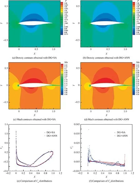
Fig. 18 Comparisons of the performances of the DG+SA and DG+ANN (Case-4).

Fig. 14 shows the comparison of the performances of the DG+SA and the DG+ANN in Case-1. Fig. 14(a) displays the Mach contours obtained using the 3rd-order DG+SA method and Fig. 14(b) shows the Mach contours computed with the 3rd-order DG+ANN method, where the Mach contours match very well and no significant difference can be observed. The pressure coefficient Cpdistributions obtained with the DG+SA and the DG+ANN also match very well in Fig. 14(c). The magnitude of the eddy viscosity near the solid boundary is very small, which make the relative error(eddy viscosityANN-eddy viscositySA)/ eddy viscositySAlarge.So relatively significant difference in some area can be observed between the friction coefficient Cfdistributions in Fig. 14(d). Fig. 14(e) and (f) give the convergence histories of the DG+SA and DG+ANN in the cases of different orders(p=0, 1, 2, 3), where all of the setups of the DG solutions remain the same for the comparisons. When p=0, it takes the same time steps (141 steps for both DG+SA and DG+ANN) to reduce the residuals down to 10-10. The p1 solutions are obtained with converged p0 solutions as the initial guesses, where the DG+SA method needs more than 6000 steps to get converged and the DG+ANN requires only 158 steps.In the cases of p=2 and p=3,it takes nearly half of the time steps for the DG+ANN to converge compared to the DG+SA. The costs of the CPU time are compared in Table 1, where the DG+ANN method is much more efficient than the DG+SA method since the ANN turbulence model is much simpler in computation than the traditional SA model and takes fewer steps to converge in high order cases. Since the p order solution starts from the converged p1 order solution,the total costs of the CPU time to obtain the p3 solutions equals to the sum of the CPU times corresponding to p=0,1,2, 3, which are 669245 s for the DG+SA and 17634 s for the DG+ANN in total.

In order to further test the generalization of the ANN model, Case-2 and Case-3 are conducted for which the Mach number in Case-2 and the attack angle in Case-3 are not covered by the training cases.The final numerical results obtained using the DG+ANN are also demonstrated with the Mach contours in Figs. 15 and 16, which agree well with those computed with DG+SA. The comparisons of the Cp, Cfand the time steps in Case-2 and Case-3 are quite similar to that of Case-1. The convergence histories are almost the same when p=0 and it takes much more steps to get converged solution when p=1 for DG+SA. When p=2 and p=3, the DG+SA needs more than double number of steps to obtain converged solution compared to the DG+ANN. The significant improvements in the efficiency of the DG+ANN are displayed in Tables 2 and 3. Fig. 17 compared the total CPU times to obtain the p3 solutions of all of the three cases.

In all of these three cases, the numerical results of the DG+ANN match well with those of the DG+SA even when the testing cases (Case-2 and Case-3) are slightly located outside the range of the training cases. The DG+ANN method converges more efficiently in all of the testing cases, which indicates that the robustness of the DG solution of RANS is significantly improved by using the developed ANN turbulence model.

In order to further test the generalization of the ANN model, the flow around a different geometry (NACA2822 airfoil, Ma=0.3, α=0°, Re=1850000) is numerically simulated, which is referred to as Case-4 here. In Fig. 18, the density contours and the Mach contours obtained with DG+SA and DG+ANN match well. Slight difference can be observed from the Cpand Cfdistributions, which is caused by the numerical error of ANN when the eddy viscosity is very small.

6. Conclusions

Because of the high-accuracy property, the high-order DG methods have been becoming more and more popular. However,the convergence efficiency is still a bottleneck when solving the RANS with complex turbulence models. In this paper, a data-driven turbulence model is developed based on an artificial neural networks, which is trained using the data from the DG solutions of the RANS with the traditional SA turbulence model.The optimal network structure is selected among a variety of candidates and further optimized by using the OBS. By evaluating the sensitivity of each input feature to the output target,four most relevant variables,ρ，ρu，ρv and ρe are chosen to construct the ANN which is embedded into the turbulence model. The resulting ANN turbulence model is tested in the framework of DG solution of RANS,where it performs as an algebraic turbulence model. Numerical results indicate that the accuracy is satisfactory. More importantly, the robustness and the efficiency of the convergence are significantly improved compared to the widely used SA model, which means that the nonlinearity of the DG discretization of the RANS is effectively reduced when using the new ANN turbulence model.

The main goal of the work is to investigate the possibility of developing a data-driven algebraic turbulence model which can improve the efficiency and the robustness of the convergence of the DG method. Although the numerical tests here only cover a small range of flow cases,the results demonstrate positive potential of developing more general data-driven turbulence models based on artificial intelligence methods in the future. A more general ANN model, which covers the cases of all Mach number and Reynolds numbers,can be considered in the future.Therefore,more training data will be needed and the structure of the ANN will need to be re-designed based on a large range of flow cases.Also,the training data in the paper was generated from the SA model which is not accurate enough for all flow cases. Data from DNS is expected to improve the accuracy of the ANN model for more flow cases.Finally,our methods selected four most relevant input features among 14 options based on the limited flow cases in this study.We expect to obtain further discoveries on the underlying mechanism of turbulence model based on data with more accuracy and more flow cases in the future.

Acknowledgements

This study was co-supported by the Aeronautical Science Foundation of China (Nos. 20151452021and 20152752033),and the National Natural Science Foundation of China (No.61732006).