Statistical delay distribution analysis on high-speed railway trains

Yuxiang Yang · Ping Huang · Qiyuan Peng · Jie LI · Chao Wen

Abstract The focus of this study is to explore the statistical distribution models of high-speed railway(HSR)train delays. Based on actual HSR operational data, the delay causes and their classification, delay frequency, number of affected trains, and space-time delay distributions are discussed.Eleven types of delay events are classified,and a detailed analysis of delay distribution for each classification is presented. Models of delay probability delay probability distribution for each cause are proposed. Different distribution functions, including the lognormal, exponential, gamma, uniform, logistic, and normal distribution,were selected to estimate and model delay patterns. The most appropriate distribution, which can approximate the delay duration corresponding to each cause, is derived.Subsequently, the Kolmogorov-Smirnov (K-S) test was used to test the goodness of fit of different train delay distribution models and the associated parameter values.The test results show that the distribution of the test data is consistent with that of the selected models. The fitting distribution models show the execution effect of the timetable and help in finding out the potential conflicts in real-time train operations.

Keywords High-speed railway · Train delay cause ·Actual operation data · Distribution model

1 Introduction

Since 2008, China’s high-speed railway (HSR) has grown significantly owing to its advantages over other modes of transportation; these include large transport capacity, low energy consumption, and high degree of punctuality.Railway passenger terminals and HSR lines have developed into networks;all these factors could improve the rail transport operations in terms of quantity and quality.

In the process of creating an HSR timetable, the conflicts between different trains over network resources should be eliminated. Ideally, trains are supposed to run according to a timetable without any conflict. However,delays are often unavoidable owing to human-related errors, interference from operating environments or facilities, and equipment-related events. Compared with road and air transportation,railways have a stricter order of line resources;that is,any delay would affect several trains and cause a series of delays.

For high-speed lines in China, once the delay is more than 1 min, the train would be marked as a delay train.According to the data from the Chinese Guangzhou Railway Corporation, during March to November in 2015, the total arrival and departure delay time are 54,327 min in Changsha station and 77,802 min in Guangzhou station.On the one hand, train delays would reduce the quality of transportation services and increase the cost of railway operations. On the other hand, they would increase the travel time of trains and cause inconvenience to passengers.Accurately analyzing the impact of the delay of HSR trains is conducive to improving the management level of HSR transportation,and is an important guarantee that HSR will provide quality transportation services to society.

The railway delay mechanism could be revealed by the delayed train records [1]. Using the actual train operation data, this paper performs a statistical distribution analysis of the HSR train delays, including the various distribution functions of train delays caused by different delay events.In particular, related parameters of these delay distributions were also estimated to describe the current delay state of the high-speed trains. The main contributions include (1) preliminary analysis of the causes of delays and the overall situation of HSR train delays as a foundation for further studies and (2) establishing distribution models and parameter estimations of delays to serve as the basis for timetabling and simulation studies of train operations.

The remainder of this paper is organized as follows.Section 2 reviews the current studies on the train operation disturbance.Section 3 introduces the structure of the delay record data.Section 4 presents the results of the causes and statistical characteristics of HSR train delays. Section 5 proposes the statistical models for the distribution of train delay time, and presents distribution model selection and parameter estimation results. Finally, conclusions are presented in Sect. 6.

2 Literature review

HSR train operation disturbance has received extensive interest, as reflected in the literature on railway transportation management, and most of the scholars have focused on the prediction of disturbance, simulation research of disturbance, and theoretical models of delay propagation. With the development of computer science and data technology, quantitative research on train performance based on operational data has become popular.However, owing to the difficulty of obtaining train operation records, most of these studies are based on simulated or partial data [2].

In the simulation and theoretical research domain, simulation software, such as LUKS [3], RailSys, and Open-Track [4], are generally used to simulate the operation of trains.However,the specific disturbance values are mostly set on the basis of qualitative methods. Keiji et al. [5]formulated a train operation simulation model for the Tokyo Metropolitan Area by taking into account the interaction between the trains and passenger-boarding model at each station. Weik et al. [6] provided a strict mathematical proof of the Strele formula for the estimation of knock-on delay.Weng et al.[7]established a regression tree model to predict train delays. This research is focused on urban rail transit; however, the operating environment of HSR is much more complex.

In terms of quantitatively studying the effects of disturbance based on data-driven methods,the existing studies focused on the distribution of the delay time. Scholars had used the lognormal, exponential, or Weibull distributions to fit the train delay duration distribution [8]. First, Schwanha¨ußer et al. [9, 10] proved that the distribution and propagation of the primary delay probability follows a negative exponential distribution. From the historical operation data of the Dutch railway, Yuan [11] found that the distribution of train arrival and departure delay fit a lognormal distribution curve. On the basis of the train operation data, Xu et al. [12] used the zero-truncated negative binomial (ZTNB) distribution to simulate and predict the probability of the daily delay in train operation.However, this research did not explain the model effect.Meng and Goverde [13] put forward an approach to reconstruct train delay propagation based on the records of the Dutch railway operation data.However,the data covers only for 1 month.

In summary,there is a growing number of studies about train delay based on actual train data. However, there is rarely statistical analysis and distribution modeling of Chinese HSR train delays. Studies of HSR train delays in China would contribute to an improvement in the management of train operation.

3 Data description

3.1 Data source

Train delay data, including data on four HSR routes, were derived from the train operation database of China Railway corporation. After removing invalid data (accounting for 4.4% of the total), which lacks the records of the delay reasons,there are still 11,452 delayed trains.That is to say,all the trains in this work are delayed trains.

3.2 Introduction to railway lines

The details about the constituent parts of the four lines, as shown in Fig. 1, are

· Beijing-Guangzhou High-Speed Railway (B-G HSR):total length of 998.5 km, from Chibi station to South Guangzhou station;this includes the lines within the 14 stations on the route and connecting lines;

Fig. 1 Schematic of four HSR lines

· Guangzhou-Shenzhen High-Speed Railway (G-S HSR): the line of 175.1 km runs from South Guangzhou station to North Shenzhen station and has five stations;

· Guangzhou-Shenzhen Intercity Railway (G-S ICR):there are six stations on the 153.4 km line from Guangzhou station to Shenzhen station;

· Shenzhen-Xiamen High-speed Railway (S-X HSR):the 362.5 km line connecting North Shenzhen station to Zhao’an station has thirteen stations.

3.3 Time period

The sample period of the delayed trains is from April 21,2014, to December 17, 2015. A sample of the data format is presented in Table 1.Here,we just consider the positive delays, meaning that trains departing and arriving earlier than their schedule time are not taken into account.

4 Analysis of train delays

4.1 Causes of delays

According to the records of the China Railway Corporation,there are over 40 kinds of events causing train delays,such as heavy rains,catenary faults,and braking equipment failures. In this article, the causes of train delays were classified into the following eleven types: human error(HE); foreign body invasion (FBI), bad weather (BW);natural disaster (ND); passenger influence (PI); vehicle fault(VF),traction and power-supply system fault(TPSF);dispatching and control system fault (DCSF); communication and signal system fault (CSSF); line fault (LF), and other problems (OP). The detailed explanations of the causes are as follows:

1. HE: unexpected maintenance (related departments require a temporary operation interruption, which is not scheduled, to maintain or examine the tracks,vehicles, or other facilities); physical discomfort of the driver; departure before the maintenance operation completed; and a stop at a neutral Sect.

2. FBI: hitting animals; pedestrians stepping on tracks;track or catenary faults.

3. BW: heavy rain, wind, or snow.

4. ND: flood, landslide, fire, or earthquake.

5. PI: temporary stop owing to passage of key trains;passenger aid; passenger transferring, and large passenger volume.

6. VF: fault in any component of a vehicle.

7. TPSF:faults of catenary,pantograph,hauling system,braking system, and so on.

8. DCSF: faults in automatic train control (ATC)system, centralized traffic control (CTC) system,Chinese train control system (CTCS), monitoring system, risk prevention system, and so on.

9. CSSF:faults of signals,transponders,communication equipment, and so on.

10. LF: faults in tracks, switches, and tunnel drainage facilities, train shaking (owing to damage to track parts), track settlement, and so on.

11. OP: faults in the air-conditioning equipment and so on.

Table 1 Format of the original data sample

4.2 Correlation analysis of the factors

The classifications of these causes for delays were based on experience. In order to explain and evaluate the classification results, the correlation coefficients between each pair of the factors were calculated.By calculating the delay time of delayed trains owing to different causes on individual days, a date-delay time matrix was obtained. The columns of the matrix are populated by the delay time because of different causes, whereas the rows contain the dates.

The results of the correlation matrix between different factors are calculated with Eq. (1) and are presented in Table 2. The largest absolute value in the correlation matrix is 0.241;this means that most factor pairs are nearly uncorrelated. These results confirm that the statistical characteristics of these individual delay factors could be considered independently.

where Xiand Xjare the delay times due to different causes on a particular day, and the subscripts i and j, which are different column numbers in the matrix, denote different causes; σXiand σXjare standard deviations of the delay time owing to different causes; and E （X ） denotes the expectation.

4.3 Overall statistical analysis of delay data

Based on different causes for delays, the overall statistical analysis of the delayed train data(see Table 3)shows that a total 1,615 delay events took place during the sample period and 11,452 trains were affected; this led to an average delay of 42 min per train.

Table 2 provides the following results. First, TPSF(19.0%) and DCSF (22.1%) have the largest probabilities of occurrence of delay; they are followed by FBI (14.9%),BW (16.8%), and VF (14.0%). These five factors accounted for 72.8%of all delay occurrences.Second,some of the low-frequency causes, such as ND and CSSF, lead to serious delays and affect a large number of trains. Third,some causes, such as ND (standard deviation of 81.23)exhibit greater randomness, and, thus, it is difficult to predict how long the disruptions will last. However, most of these factors generally lead to regular delays; for example, TPSF has a standard deviation of 26.78. Finally,81.0%of the delays last for less than 60 min,while 90%of the delays are less than 91 min.A kurtosis of 90.60 for the train delays and a huge gap between the maximum delay(1199 min)and the 75 percentile delay(49 min)prove that the distribution is biased to the left as shown in Fig. 2).

4.4 Chronological analysis of delays

The total delay time and the number of delayed trains are calculated for each day of a 2-year period, as shown in Fig. 3;owing to holidays and festivals,the peaks are nearly coincident.In February, May, and October,there are some grand holidays and festivals, such as Spring Festival and National Day in China. On these days, there is huge demand for transportation. More high-speed trains are dispatched, even at night, and the regular midnight maintenance is skipped to transport more passengers. The lack of maintenance and large train density lead to more infrastructure-related faults, and more trains are affected when disruptions occur. Second, delays take place more often in spring and summer, because the operating environment is worse in these seasons. More heavy rains and winds in these seasons cause more damage of exposed equipment, and limit train speed.

Table 2 Correlation matrix between various factor pairs

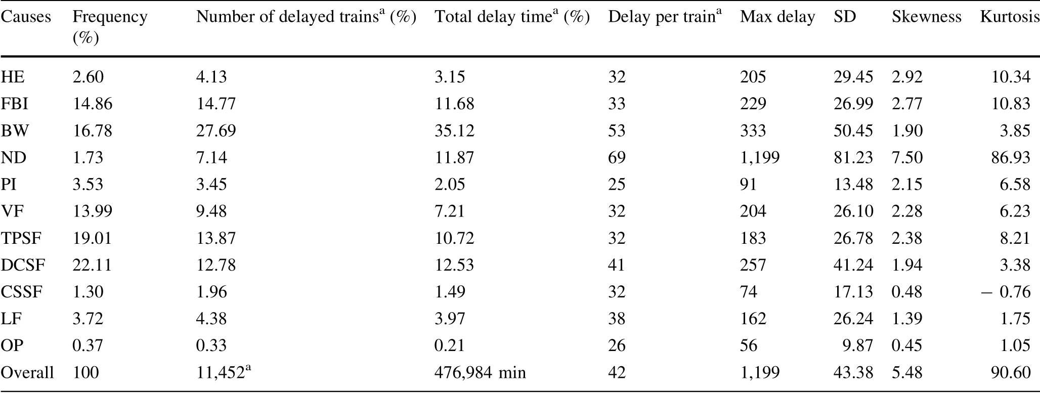
Table 3 Overall statistical analysis of delayed train data

Fig. 2 Number of delayed trains along with delay time

5 Distribution intensity and parameter estimations

To evaluate a timetable or add disturbance events in the simulation process of train operations, it is necessary to consider the intensity of disruptions or disturbances. The intensity, on the one hand, means the number of delayed trains in a time period.On the other hand,it also stands for how long the delay event lasts.

5.1 Duration distribution of delayed trains in given time period

Primary delay probability has been proved to follow a negative exponential distribution [14-16].

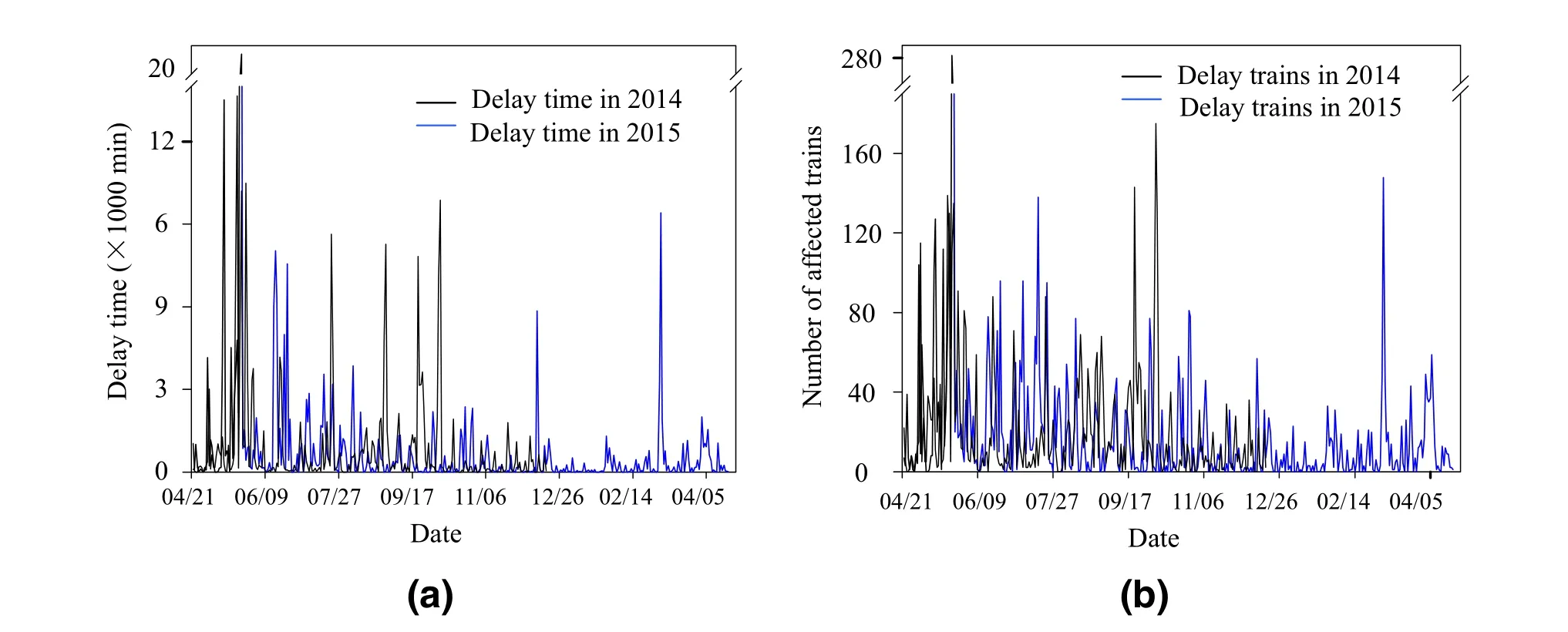
Fig. 3 Total delay time (a) and the number of delayed trains (b) on individual days

where λ is the rate parameter.

In addition, a zero-truncated negative binomial distribution (ZTNB), as expressed in Eq. (5), was applied to model and forecast the probability of the number of delayed trains per day [12]:

where α is the over-dispersion parameter; γiis the estimated number of delayed trains for the ith observation and FNB（yi） is the probability of negative binomial distribution when the frequency is yi[12].Moreover, γiis calculated as

where xniis the frequency of the ith cause.

5.2 Distribution of delay duration

A specific distribution should be selected to model the possible delay duration for a train.The data collected from April 21st,2014 to December 17th,2015 were divided into two groups: the first 12 months (7,872 or 68.7% of the observations,or the so-called modeling data)were used for establishing the model and parameter estimation, and the following 8 months (3,580 or 31.3% of the observations;so-called testing data) for the hypothetical test and calculating the relative values of goodness of fit. All the calculation processes subsequent were implemented on the R-project program.

5.2.1 Selection of candidate distributions

One of the typical causes,bad weather(BW),was taken as an example to explain the method for candidate distribution selection.

First, the empirical density histogram, nuclear curve,and cumulative distribution of BW were used to intuitively determine candidate distributions. As shown in Fig. 4, the majority of the delay durations were less than 100 min,presenting a left-skewed distribution.

In addition, Cullen-Frey graph (Fig. 5) were introduced to quantitatively compare the skewness and kurtosis of the target dataset and the candidate distributions.Owing to the uncertain distribution and skewness and kurtosis values of the dataset,a nonparametric bootstrap was performed in the Cullen-Frey graph by using the argument boot [17]. Some of the distributions (normal, logistic, etc.) have only one possible value for the skewness and kurtosis, while others(lognormal, gamma, and beta) have areas of possible values,presented as lines or areas.Based on the result of BW in Fig. 5, with a positive skewness and a kurtosis not far from 5 [18], three types of distributions were taken into account: lognormal, exponential, and gamma. With the same analysis and calculation for all the causes, Table 4 shows the results of candidate distributions for the remaining causes of delay.

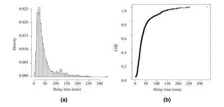
Fig. 4 Histogram (a) and cumulative distribution function (b) plots of bad weather

Fig. 5 Cullen and Frey graph with a bootstrapped value of 1,000 for BW data

Table 4 Candidate distributions for different causes

5.2.2 Parameter estimation by maximum likelihood estimation (MLE)

After confirming the candidate distributions,suitable fitting and parameters of the distribution models were needed.Figure 6 presents the comparison of the candidate distributions of BW by four classical goodness-of-fit plots [19].As these plots show,the lognormal distribution might be a suitable choice for BW.In the Q-Q plot,none of the three types of candidate distributions fit the tail well.

For quantitative analysis of the best fitting distribution,the maximum likelihood estimation(MLE)method is used.The probability density functions of lognormal, exponential, and gamma distributions are as follows:

where μ and σ are the logarithmic mean and standard deviation of the variables.

where λ is the rate parameter that represents the frequency of events.

where α is the shape parameter and β is the scale parameter.

Maximum likelihood equation is defined as

where （x1，x2，x3，···，xn）is the sample data set and θ is the unknown parameter set. Acould maximize L （θ ） or ln L（θ ） should be found. For example, in case of a lognormal distribution, the likelihood function is

where C is a constant.

The estimated parameters are:

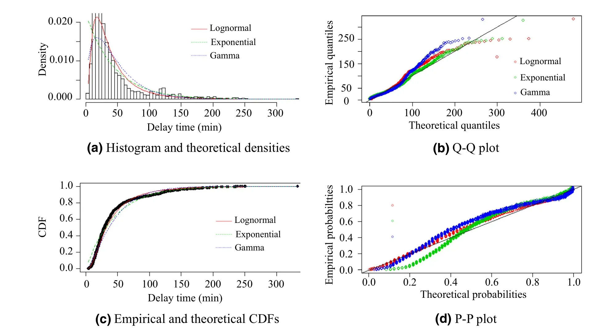
Fig. 6 Four types of plots for comparing the candidate distribution for BW. A density plot gives the shapes of the original and candidate distributions through a histogram; a CDF plot shows the fit of the cumulative distribution functions; a Q-Q plot and a P-P plot present the goodness of fit of the candidate distribution

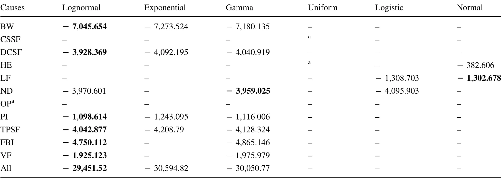
Table 5 Results of ln L（θ ） according to the candidate distributions of causes

By calculation,the maximum ln L（θ ）values of BW are- 7,045.654 (lognormal distribution), - 7,273.524(exponential distribution), and - 7,180.135 (gamma distribution). Lognormal distribution has the maximum ln L（θ ） value; thus, it is the most suitable distribution. In this case, μ = 3.469 and σ = 0.793. Therefore, the probability distribution function for the delay of one train caused by BW is as follows:

The estimated results of ln L（θ ） of the candidate distributions for different causes are shown in Table 5.The bold numbers are the maximum values,indicating thatthe distribution has the best fit. In addition, not every distribution has an MLE value. Table 6 shows the estimated parameter results of the best distributions.

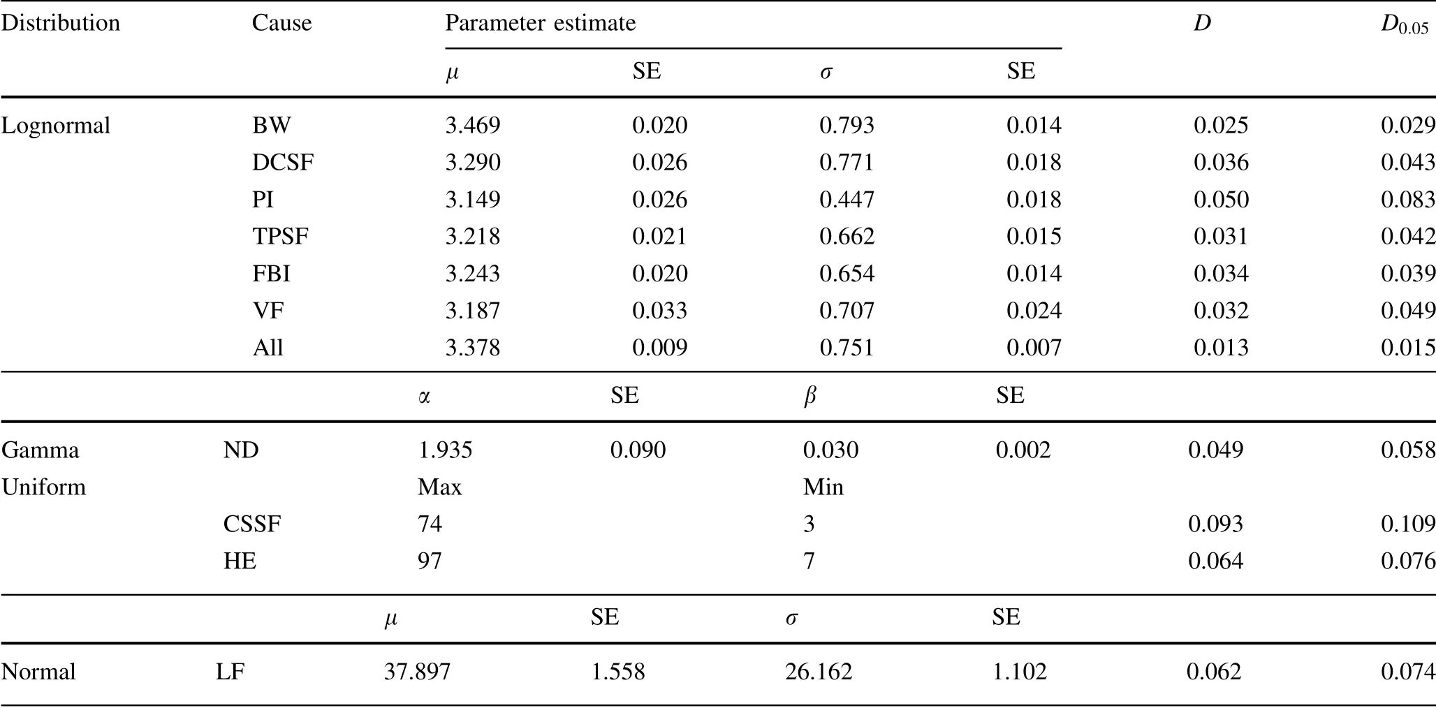
Table 6 Parameter estimate results of the best distributions

5.2.3 Model testing

The Kolmogorov-Smirnov test (K-S) [20] is used to evaluate these distributions. As shown in Eq. (13), the statistic is the maximum difference between the empirical piecewise function of the dataset and the empirical distribution function of a theoretical distribution. In this paper,the significance level of the test is 0.05, and the critical value of D is calculated by Eq.(14)when the sample size is large enough (generally greater than 50). According to the K-S test, if D is not greater than D0·05, the null hypothesis(H0)is accepted.The null and alternative hypotheses in the test are defined:

H0 Delay time data fitting the identified distribution;

H1 Delay time data not fitting the identified distribution.

where F1（x ） and F2（x ） are the empirical distribution functions of the modeling dataset and the candidate distribution, respectively, and m is the sample size.

The modeling data were applied to conduct the K-S test;because all the models passed the K-S test, the nullhypothesis (H0) is accepted. Subsequently, the testing of fitting models was calculated. Using the same method, the testing data were introduced to match the specified probability distributions of every cause by the K-S test. The results are listed in Table 7.

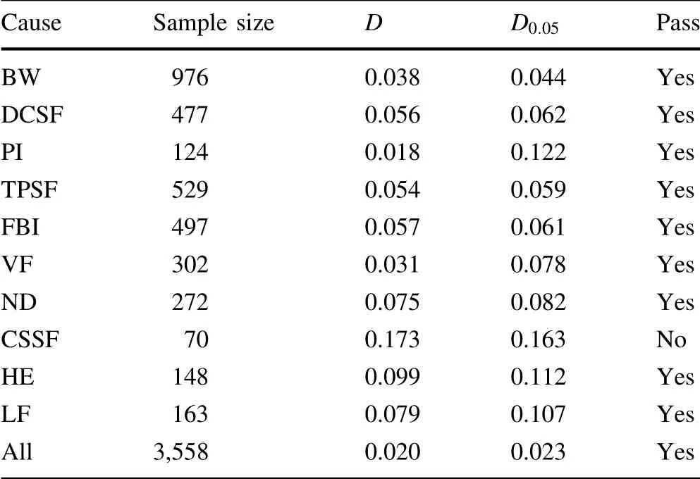
Table 7 Results of the K-S test for testing data

The test results show that the distribution models fitted in this paper all passed the K-S test,except for CSSF.The model could accurately describe the general law of HSR disturbance affecting the train delay time distribution, and has good prediction ability and practical application.As for CSSF, the reason might be (1) the data scale is not adequate for the precise calculation and (2) the probability of its occurrence is too random, and, thus, the uniform distribution cannot be accurately fitted.

6 Discussion and conclusions

In this paper, the statistical train delay status and distribution models of HSR were investigated by using the actual operational data. Based on the categorization of delay events, different distribution models were fitted and the related parameters were estimated. The main findings and contributions are as follows:

1. Based on the actual performance of the trains on highspeed lines, the train operation delay status were extracted and analyzed.

2. Distributions of delay time were modeled for eleven causes for delay,and all the most suitable fittings were screened by the MLE method and K-S test.

3. The models were checked with the operation data.The test results show that most of the distribution models fitted in this paper had good practical applicability,and could accurately fit the impact of HSR disturbance on train delay time, which had great practical application value.

AcknowledgementsThis work was supported by the National Key R&D Plan (No. 2017YFB1200701) and National Nature Science Foundation of China (No. U1834209 and 71871188). We acknowledge the support of the Railways Technology Development Plan of China Railway Corporation(No.2016X008-J).Parts of the work were supported by State Key Lab of Railway Control and Safety Open Topics Fund (No. RCS2019K007). We are grateful for the contributions made by our project partners.

Open AccessThis article is distributed under the terms of the Creative Commons Attribution 4.0 International License (http://creativecommons.org/licenses/by/4.0/), which permits unrestricted use,distribution,and reproduction in any medium,provided you give appropriate credit to the original author(s) and the source, provide a link to the Creative Commons license, and indicate if changes were made.