Targeted local angle-based multi-category support vector machine*
2019-07-26KANGWenjiaLINWenhuiZHANGSanguo
KANG Wenjia, LIN Wenhui, ZHANG Sanguo†
(1 School of Mathematical Sciences,University of Chinese Academy of Sciences, Beijing 100049, China;2 Technology Research Institute, Aisino Corporation, Beijing 100195, China)
Abstract The support vector machine(SVM) is one of the most concise and efficient classification methods in machine learning. Traditional SVMs mainly handle with binary classification problems by maximizing the smallest margins. However, the real-world data are much more complicated. On the one hand, the label set usually has more than two categories, so SVMs need to be generalized for solving multi-category problems reasonably. On the other hand, there may exist one special variable which should be singled out to preserve its effect on the final results from other variables such as age in bioscience field. We name such a special variable as targeted variable. In this work, in order to take both aspects mentioned above into consideration, targeted local angle-based multi-category support vector machine(TLAMSVM) is proposed. This new model not only solves multi-category problems but also pays special attention to targeted variable. Moreover, TLAMSVM solves multi-classification in the framework of angle-based method, which provides a better interpretation from the geometrical viewpoint, and it uses local smoothing method to pool the information of targeted variable. In order to validate the classification effect of TLAMSVM model, we apply it to both simulated and real data sets, respectively, and get the expected results in numerical experiments.
Keywords local smoothing; multi-category support vector machine; angle-based maximum margin classification framework
Machine learning, as a new research orientation, plays a significant role in the age of big data. A widely used classification method of machine learning is support vector machine(SVM)[1]. It is a kind of classic margin-based classifier, which seeks for the most appropriate hyperplane in the feature space and solves the optimization problem in the form of (loss+regularization)[2]. In the last decades, SVM and its derived algorithms have held an important place in many fields[3]on account of its perfect prediction accuracy and computational efficiency.

Apart from expanding the numbers of category for SVM, researching the interrelation of covariant variables is a worthy direction to study as well. For example, SVM is a popular algorithm in disease research to predict disease risk status of patients. However Wei et al.[11]mentioned that some variables themselves might make little contribution to prediction but play significant roles when they are coordinated with other correlated variables. So the method that uses local linear smoothing SVM on the entire feature variable space is proposed by Ladicky and Torr[12]. Since it does not accomplish smoothing technique successfully in high-dimensional feature space, Chen[13]developed a targeted local smoothing kernel weighted support vector machine (KSVM), which only needs the data in targeted dimension to be plentiful. It achieves an age-dependent prediction rule to discriminate disease risk via optimizing a kernel weighted problem. It gets quite good results on binary classification problems. It is worth applying such a local weighted tool to MSVM.
In this study, we mainly make two contributions. Firstly, we combine angle-based multi-category classification framework of RAMSVM model and targeted local smoothing method of KSVM model, and propose a new MSVM model, targeted local angle-based multi-category support vector machine(TLAMSVM), which offers a better classification prediction for certain data sets. Secondly, TLAMSVM model provides more detailed analysis for a sample according to its value of targeted variable. Before introducing TLAMSVM model, some fundamental knowledge of RAMSVM model and KSVM model will be described in section 2, which are the basis of TLAMSVM model. In section 3, the detailed presentation of TLAMSVM model will be shown, followed by its computational process of coordinate descent method. In section 4, we will show some experimental results in four simulated and real data sets and give some illustrations to demonstrate the strengths of TLAMSVM model. At the end, we will conclude the article with discussions in section 5.
1 Background and related work
1.1 Reinforced angle-based multi-category support vector machine(RAMSVM)
As for k-class data sets, the angle-based large-margin classification framework defines a k-vertex simplex in (k-1) dimensional space,W1,W2,…,Wk, which correspond to each class,
whereWjrepresents thejthvertex,j=1,2,…,k,1represents the vector where each element is 1,ejrepresents unit vector where every element is 0 except for thejthone.Wj,1,ej∈k-1. It can be verified that ‖Wj‖=1 and the angle between any two adjacent vectors is equal. Each observationxcould be mapped to (x)=(f1(x),…,fk-1(x))∈k-1. Consequently, there are k angles ∠(f(x),Wj), and we regard argminj∈{1,…,k}∠(f(x),Wj) as the predicted category. It is equivalent to write this prediction rule as
According to the regular form of a large-margin classification algorithm, we add a penalty termJ(·) to the loss function. So the optimization problem becomes

(1)
herel(·) is a loss function, which measures the cost of wrong predictions. Nevertheless, typical loss function such as hinge lossl(u)=[1-u]+is not Fisher consistent. Inspired by Lee[7], RAMSVM uses a convex combination of loss function to overcome this drawback. Therefore (1) is turned into
γ[(k-1)-〈f(xi),Wyi〉]+}+λJ(f),
(2)
hereγ∈[0,1] is the convex combination parameter. It has been proved that, whenγ∈[0,0.5], the loss function of RAMSVM model is Fisher consistent[10]. In addition, whenγ=0.5, RAMSVM is stable and almost reaches the optimal classification accuracy. Therefore we defaultγ=0.5 directly in the latter work.
1.2 Kernel weighted support vector machine(KSVM)
Take binary medical data as an example, letYdenote the set of labels {1,-1}, which represents whether a subject is at the disease risk or not. Let “age” be the targeted variableU, and variableXcontains other features. Now the purpose is to train a classifier which depends on age information. Firstly, we consider making some changes on typical discriminant score as follows:
α(U)+XTβ(U),
(3)
whereα(U) is a baseline without specific functional form,β(U) is a vector whose elements represent the coefficients ofXthat varies with age. It is common sense that the subjects with similar ages and other features would also have similar disease risk. So when changing ageUsmoothly,β(U) varies smoothly too. Some features might provide more information for classification when age is larger while others do reversely. From this perspective, people would have better understanding of each physical sign. Then, after calculating the value in (3), the one with a negative score will be classified as risk-free and the one with a positive score will be classified to risk group.
After choosing an appropriate loss function, the targeted local smoothing kernel weighted support vector machine (KSVM) model trains a classifier via solving
l{Yi,Xi;α(u0),β(u0)}+λ‖β(u0)‖,
whereKhn(·) is kernel density function, which could pool information of subjects whose ages are aroundu0within certain bandwidthhn. In another word, KSVM model trains different SVMs at everyu0, respectively, and the weight of theithsample isKhn(Ui-u0).

2 Methodology and computation
In this section we firstly illuminate how to design multi-category local smoothing kernel weighted optimization problem in TLAMSVM model. Then we list out some main computational steps of TLAMSVM model using coordinate descent method. We take linearly separable case as example, since to non-separable case, we can use kernel trick.
2.1 Targeted local angle-based multi-category support vector machine(TLAMSVM)

X=(X1,X2,…,Xn)=(1,X(1),X(2),…,X(p))T.
(4)
Assume the classification function vector atU=u0is
fq(u0,X)=XTβq(u0) (q=1,…,k-1),
(5)

(6)
where the {(1-γ)∑j≠yi[1+〈f(u0,Xi),Wj〉]++γ[(k-1)-〈f(u0,Xi),Wyi〉]+} is the loss function of our model, and the weight before loss of each observation,Khn(Ui-u0), is smoothing kernel function with bandwidthhn, like that of KSVM model. Considering the more general situation, we bring in the concept of “soft margin” to allow part of samples dissatisfying constrain
-〈f(u0,Xi),Wj〉>1 and 2-k+
〈f(u0,Xi),Wyi〉>1,
that is to say, put slack variablesξi,j(ξi,j≥0) into constrains, and we get
-〈f(u0,Xi),Wj〉>1-ξi,j, (i=1,…,n),
2-k+〈f(u0,Xi),Wyi〉>1-ξi,j,
(i=1,…,n,j≠yi).
(7)


(8)
Obviously, (8) is a constrained optimization problem, whose Lagrangian function could be defined as
[ξi,j-〈f(u0,Xi),Wj〉-1].
Hereαi,jandτi,jare Lagrangian multipliers. After simplification, we get


(9)
whereAi,j=Khn(Ui-u0)[γI(j=yi)+(1-γ)I(j≠yi)].
Let the last two parts of (10) asL1andL2,
Take partial derivatives ofLwith respect toβq(u0) andξi,j, then let the partial derivatives be zero,
(i=1,…,n;j=1,…,k),
(10)

(11)
From (12) one obtains

(12)
and then obtains
We get

(13)
Pluging (10), (11), and (13) in (9), we simplify Lagrangian function as

(14)
Pluging (12) in (14) and maximizing Lagrangian function, we get a new form of that,
s.t. 0≤αi,j≤Ai,j.
(15)
2.2 Computation using coordinate descent method
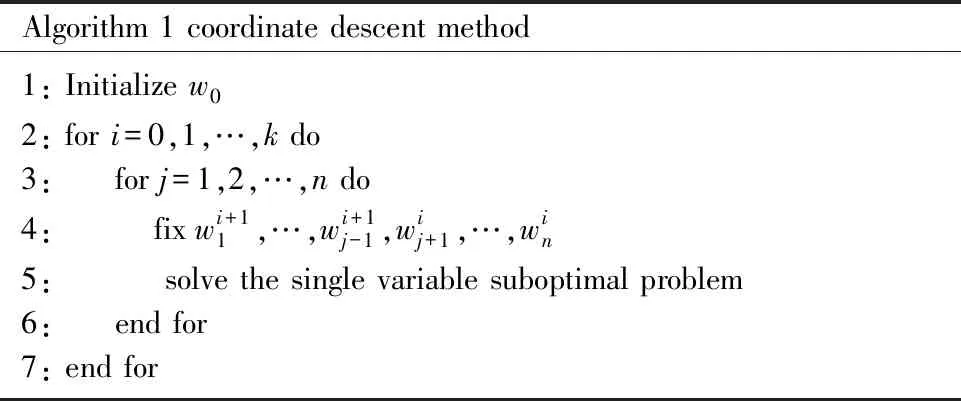
Coordinate descent (CD) method is a remarkable tool to solve large-scale data problems. It is mainly used to solve the convex optimization problems. It treats each dimension of the solution vector of the optimization problem as a coordinate, and selects one-dimensional coordinate for iterative optimization. The iterative process consists of the outer loop and the inner loop. In each outer loop, the inner loop optimization can be considered as a single variable sub-optimization problem, and only one scalar solution needs to be optimized at a time.
Assume thatw∈nis the solution vector of an optimization problem. We set a total ofkiterations. Beginning with initializedw0, we will getw1,w2,…,wkin turn. Regarding each iteration as an outer loop, each of that will iterate on each dimension ofw=[w1,w2,…,wn]. So here each outer loop containsninner loops. Fromithouter loop andjthinner loop,wi,jcan be generated,
Notice thatwi,1=wiandwi,n+1=wi+1. Updatewi,jintowi,j+1through solving single variable subproblem
whereej=[0,…,0,1,0,…,0]T. At inner loop, many tools can be used, such as Newton method and CMLS.
Now we present the computational procedure of TLAMSVM using coordinate descent method.
Algorithm 1 coordinate descent method1: Initialize w02: for i=0,1,…,k do3: for j=1,2,…,n do4:fix wi+11,…,wi+1j-1,wij+1,…,win5: solve the single variable suboptimal problem6: end for7: end for


Therefore, in them+1thstep, =1,…,n,j=1,…,k-1,l=1,…,p, we set

(16)
Step 3. Repeat above until all estimated values are convergent.
Classification function vector is
f(u,X)=(f1(u,X),f2(u,X),…,fk-1(u,X)).
Therefore, any new sample (u′,X′) will be mapped intof(u′,X′) and formkangles with vertex vectors ∠(f(u′,X′),Wj). Then we assign its label as
3 Numerical study
In this section, we use numerical experiments to verify the effect of TLAMSVM model and choosef1score to measure its classification result.f1score is a common criterion in binary classification problems. In this paper, we generalizef1score to measure multi-category cases. In detail, we compute correspondingf1score for each class by viewing current class as positive one and the rest as negative one, the average of allf1score is the final result for classifier.
It is worth noting that when dealing with non-linear problems, TLAMSVM model needs both Mercer kernel functionK(·) and local smoothing kernel functionkhn(·). The difference is obvious, the former is used to construct non-linear decision boundaries, while the latter is used to aggregate information nearu0. In numerical experiments, we use linear Mercer kernel, gaussian Mercer kernel and polynomial Mercer kernel as Mercer kernel function. And uniform kernel, gaussian kernel and Epanechikov(short as ep) kernel function as local smoothing kernel function.
3.1 Simulation results
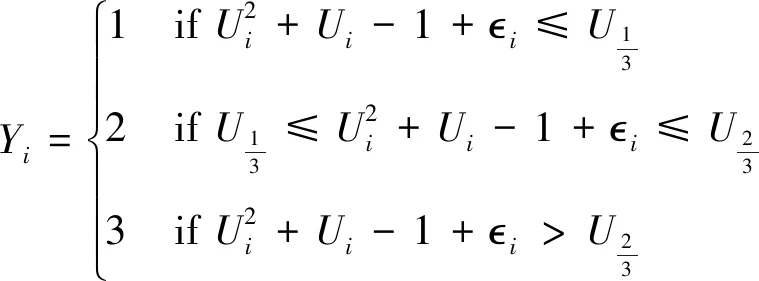
We generate two simulated data sets:S1andS2. Data inS1has 1 000 samples with 3-class label and 3 features. Data inS2has 1 500 samples with 5-class label and 7 features. We carry out 10 simulation runs for each setting and the final results are averaged values. We generate targeted variableUifromU(0,1) for bothS1andS2. And the label ofS1is defined as (17). As forS2, we use the same method to generate label, due to limitation of space, the formula wouldn’t be listed in this article.
(17)

Xi|Yi,Ui~MVN{β(Ui)Yi,σ2I}
whereβ(u)=(sin(4πu), 2e-20(u-0.5)2)T
As forS2, we generate featuresXi=(Xi1,Xi2,Xi3,Xi4,Xi5,Xi6)Tfrom andσ=2
Xi~MVN(μ(k)η(Ui)I{Xi∈classk},σ2I)

(18)
μ(1)=(5,5,0,0,0,0),μ(2)=(0,5,5,0,0,0)
μ(3)=(0,0,5,5,0,0),μ(4)=(0,0,0,5,5,0)
μ(5)=(0,0,0,0,5,5)
We mainly compare effects of three models: KMSVM, RAMSVM and TLAMSVM. KMSVM is a multi-category generalization form of KSVM, it combines the OvO multi-classification framework with KSVM method. While RAMSVM doesn’t use varying-coefficient model and regards targeted variable as a common feature. Both TLAMSVM and RAMSVM use angel-based multi-category framework. In each model, we utilize 5-fold cross validation to determine parametersλandhn.
Table 1 and Table 2 record the effects of model RAMSVM and TLAMSVM on simulated dataS1andS2.

Table 1 Comparison of f1 score between RAMSVM and TLAMSVM on data set S1
Since RAMSVM model does not need to use local smoothing kernel function to build many MSVMs according to targeted variable, it has advantage of computation time. But as for predictive accuracy, TLAMSVM model still has a better performance no matter we use which Mercer kernel or local smoothing kernel function.
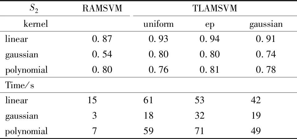
Table 2 Comparison of f1 score between RAMSVM and TLAMSVM on data set S2
Table 3 and Table 4 recordf1scores and training time of KMSVM and TLAMSVM model on simulated dataS1andS2.
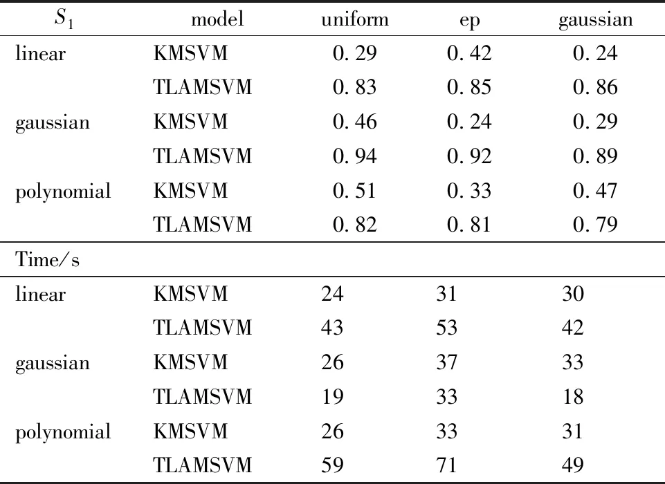
Table 3 Comparison of f1 score between KMSVM and TLAMSVM on data sets S1 and S2
TLAMSVM model provides a better prediction than KMSVM model with same Mercer or local smoothing kernel function and similar training time. The values in Table 5 are the average results of prediction of model RAMSVM and TLAMSVM onS1.
Here we compare three cases, which have different feature space respectively,Xi1only,Xi2only and both of them. We find that thef1score of TLAMSVM model is much larger than that of RAMSVM model when using single feature variable.

Table 4 Comparison of f1 score between KMSVM and TLAMSVM on data set S2
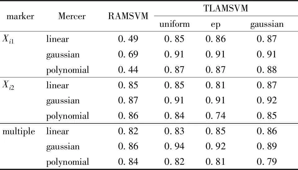
Table 5 Comparison between RAMSVM and TLAMSVM on data set S1
So TLAMSVM model does not rely on the number of feature variables in model so much as RAMSVM model does. Likewise, TLAMSVM model has better results with any kernel function in three cases.
3.2 Real data analysis
In this subsection, we demonstrate the classification effects of TLAMSVM model via using two real data sets, Cervical Cancer data and Protein Localization Sites data, named asD1andD2. Both of them are from University of California Irvine machine learning repository website. The Cervical Cancer data is derived from Universitario de Caracas Hospital. It is collected from 858 patients and it includes demographic information, patients’ habits and their historic medical records. The Protein Localization Sites data is derived from a research about an expert system, which uses the information of the amino acid sequence and source origin to predict localization sites of protein. It has 1 484 samples and 10 categories.
3.2.1 Application to Cervical Cancer data set
Cervical cancer remains one of the leading causes of death among patients with malignant gynecologic disease. It could be caused by a number of factors, for instance, viral infection, the number of sexual behavior, the number of pregnancies, smoking habits etc. From the viewpoint of Computed Aided Diagnosis System, there are several diagnosis methods in the detection of pre-cancerous cervical lesions. Here are the four most frequently-used methods in examination, colposcopy using acetic acid-Hinselmann, colposcopy using Lugol iodine-Schiller, cytology and biopsy[14]. The data set records the results of these four tests(Hinselmann, Schiller, cytology and biopsy). From these four tests results, we generate artificially a response variabley∈{1,2,3} that reflects the confidence of the diagnosis. When all of the four test results are normal,y=1, when the results of any one or two test are normal,y=2, andy=3 for rest situations. Then we get a 3-category data set.
After some common data preprocessing procedures, we get a data set without missing data nor outliers. And we reduce the number of variables in model from 31 to 12 by calculating the conditional information entropy and information gain of each variable. And we regard feature “age” as targeted variable in this data set. Due to the special property of data, we consider use a combination of undersampling and oversampling techniques (ENN+SMOTE) as balancing tool to process training data. The principle of ENN is to remove the samples whose class is different from class of the majority of its k-nearest neighbor. SMOTE[15]is a relatively basic oversampling method that reduces the differences of number between different categories. For each sample of the minority class, connect this sample between the nearest k samples of it with same category, then there will be k lines, generate one sample randomly from each line, then get k new samples of the minority class.
Table 6 is the numerical results of model TLAMSVM and RAMSVM with different Mercer kernel functions and local smoothing kernel functions on cervical cancer data set. It can be seen that, when using the same local smoothing kernel function, the polynomial Mercer kernel has the best classification accuracy. With the same Mercer kernel function, the Epanechikov and gaussian local kernel function has the relatively better prediction performance. Comparing the average accuracy of TLAMSVM model, the average prediction effect of TLAMSVM model is slightly better than that of RAMSVM model.

Table 6 Summary of accuracy of TLAMSVM and RAMSVM on Cervical Cancer data set
We can get the corresponding estimated coefficientβ(u) for any given value of targeted variableu. Figure 1 is the line chart of the coefficient in the first dimension, it shows the variation trend of each coefficient corresponding to 5 feature variables as “age” changes.

Fig.1 β1(u) vs. the targeted variable (age) on D1
From Fig.1 we can see, the influence of feature “Smokes” is small when age is between 20 and 40, but it increases a lot when age becomes larger. It means when facing the young patients, the information about his or her smoking habit is not as important as other variables. However, when judging the middle-aged patients, their smoke habit could offer more information for classification.
Figure 2 describe the inner product of classification function vector of sample and each simplex (〈f(x),Wj〉, (j=1,2,3)) when targeted variableUtakes different values.
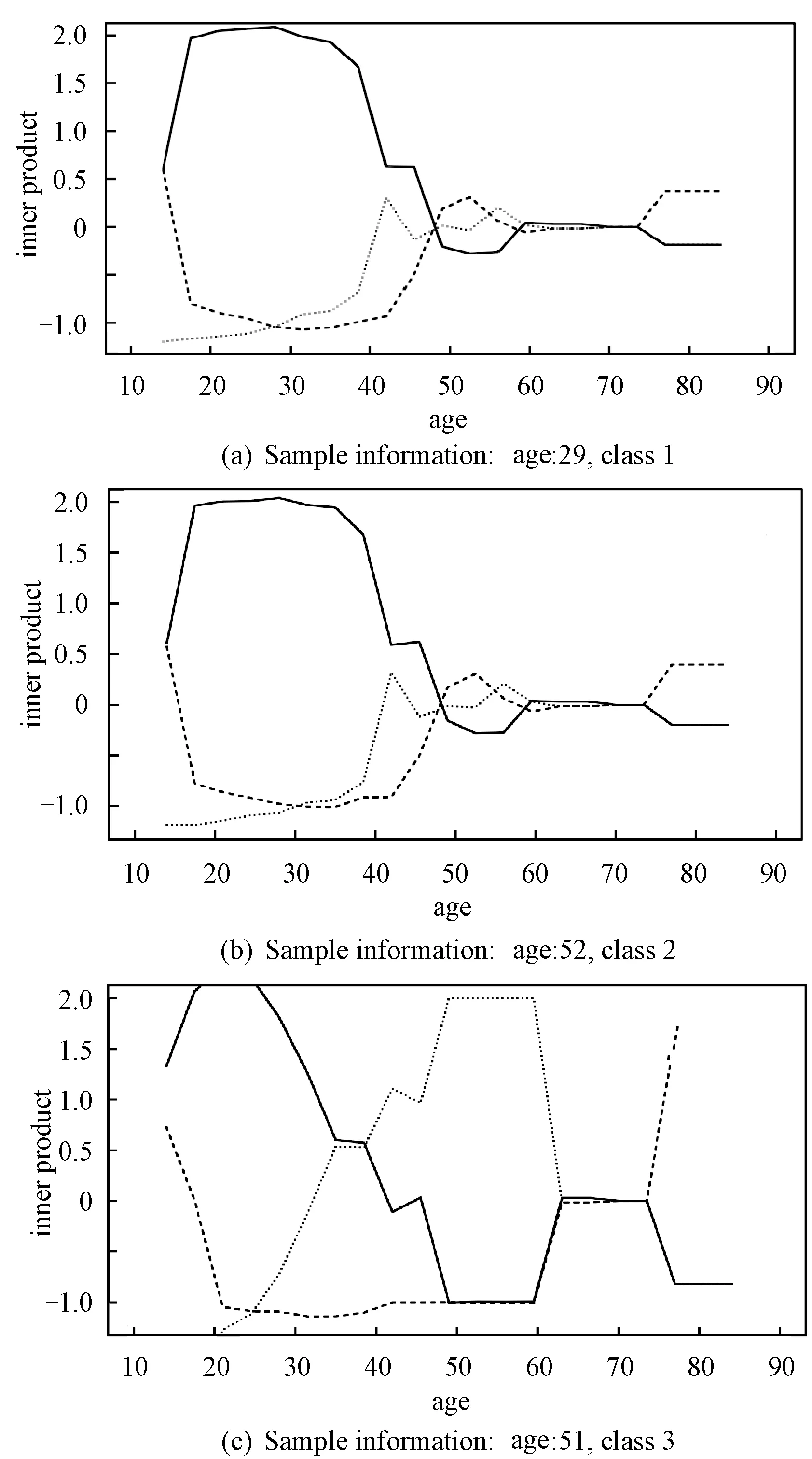
solid 〈f(x),W1〉, dashed: 〈f(x),W2〉, dotted:〈f(x),W3〉.Fig.2 Predictions for the three given samples on D1
From Section 3 we know that the sample will be classified to the category which has the maximal inner product value. So at any fixed age, the class which the top line corresponds to is the prediction result. Fig.2 reflects that different value for the targeted variable will affect final classification result of 3 given samples. These three subgraphs are the prediction details of three samples, which belong to the class-1, class-2 and class-3 respectively. The age of these these samples are 29, 52, 51 in sequence.
Firstly, we can find that TLAMSVM model gives the correct prediction according to the prediction rules. Secondly, for identical feature variables, different values of the targeted variable will affect the result of determination for that sample. That is to say, with fixed other physiological characteristics, if we assume that the patient is at different ages, it would come out different diagnosis results. Take the third sample as an example, the patient is 51 years old and the true label is 3, which means the patient has high-risk of suffering from cervical cancer. However, we would give an entirely different judgement if we regard the same physiological characteristics values as information from a patient with other age. Patient whose age is from 20 to 30, would be diagnosed as the class-1(no cervical cancer), and patient whose age is over 75, would be diagnosed as class-2(no confirmed). Thus it can be observed that the TLAMSVM model can accurately grasp the essential information of the sample by studying the relationship between the targeted variable and other feature variables to provide better prediction.
3.2.2 Application to Protein Localization Sites data set
Protein Localization Sites data set has 8 features, which are scores of some methods for measuring information about protein or amino acid. It has 10 classes to represent the different localization sites of protein, such as CYT(cytosolic or cytoskeletal),NUC(nuclear),MIT(mitochondrial) etc. We use model RAMSVM and TLAMSVM to train data and get classifiers.
Figure 3 is based onD2(Protein Localization Sites data).

solid: feature ‘gvh’, dashed: feature ‘alm’, dotted: feature ‘mit’,dashed-dotted: feature ‘nuc’.Fig.3 Estimated values for the coefficients of the first three dimensions on D2
And we set “mcg”(McGeoch’s method for signal sequence recognition) as targeted variable. Because of limitations of space, Fig.3 only demonstrates the coefficientβ(u) in the first, second and third dimension. And these subgraphs are enough to show the variability of coefficients in model TLAMSVM.
Figure 4 is the inner product graph for a certain sample, whose feature “mcg” equals to 0.45 and real label is class-1. From Fig.4, we know that the TLAMSVM model gives a correct prediction (class-1) for this sample, and the classification results would be different if the “mcg” value of this sample was different.
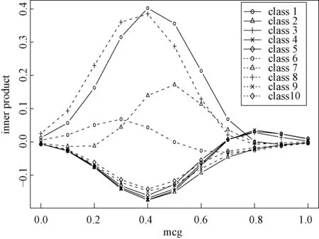
Fig.4 Predictions for a given sample under different targeted variables (mcg) on D2
Table 7 records the effect of TLAMSVM and RAMSVM model on Protein Localization Sites data set. From Table 7 we can get the same conclusion as Cervical Cancer data. The classification accuracy of TLAMSVM model is better than that of RAMSVM model, consistent with the simulation results. And we can get the same result of classification prediction from the model and its prediction rule.

Table 7 Summary of accuracy of TLAMSVM and RAMSVM on Protein Localization Sites dataset
4 Discussion
In this study, TLAMSVM model is proposed to solve multi-category classification problems and make a better prediction for different samples. In numerical experiment section, we firstly predict the risk of disease and show its dependency on the age. Building age-specific predictive model helps to study the appropriate time of intervention and find potential features which provides individualized treatment for a certain disease. The fitting coefficientβ(u) describes the age sensitivity of each feature variable to disease risk. Then we obtain good results on protein localization sites data and make a more “personalized” prediction for samples whose “mcg” values are different. Finally, the simulation results and real data analysis show that the different selections for Mercer kernel and smoothing kernel functions may lead to minor differences in prediction accuracy.
We consider the feature variables with the targeted variable dependency, but it is easy to ignore the features which have stable effect. Thus, we will add some features with invariant effects to the initial classification function in future work, likeα(U)+XTβ(U)+ZTγ.
