A Self-Organizing Memory Neural Network for Aerosol Concentration Prediction

Qiang Liu ,Yanyun Zou and Xiaodong Liu

Abstract: Haze-fog,which is an atmospheric aerosol caused by natural or man-made factors,seriously affects the physical and mental health of human beings.PM2.5(a particulate matter whose diameter is smaller than or equal to 2.5 microns)is the chief culprit causing aerosol.To forecast the condition of PM2.5,this paper adopts the related the meteorological data and air pollutes data to predict the concentration of PM2.5.Since the meteorological data and air pollutes data are typical time series data,it is reasonable to adopt a machine learning method called Single Hidden-Layer Long Short-Term Memory Neural Network(SSHL-LSTMNN)containing memory capability to implement the prediction.However,the number of neurons in the hidden layer is difficult to decide unless manual testing is operated.In order to decide the best structure of the neural network and improve the accuracy of prediction,this paper employs a self-organizing algorithm,which uses Information Processing Capability(IPC)to adjust the number of the hidden neurons automatically during a learning phase.In a word,to predict PM2.5 concentration accurately,this paper proposes the SSHL-LSTMNN to predict PM2.5 concentration.In the experiment,not only the hourly precise prediction but also the daily longer-term prediction is taken into account.At last,the experimental results reflect that SSHL-LSTMNN performs the best.

Keywords: Haze-fog,PM2.5 forecasting,time series data,machine learning,long shortterm memory neural network,self-organizing algorithm,information processing capability.

1 Introduction

PM2.5(a particulate matter whose diameter is smaller than or equal to 2.5 microns)is one of the most critical factors for haze-fog formation.PM2.5emissions can be divided into primary pollution sources and secondary pollution sources.The primary pollution sources are mainly PM2.5particles produced directly by the combustion of fossil fuels(petroleum,coal,etc.),biomass fuels(straw,wood),dust and so on.Secondary pollution sources are mainly PM2.5particles produced by the combination of volatile organic compounds(VOCs),nitrogen oxides,sulfur dioxide,hydrocarbon organic compounds,nitrates and other particles in the atmosphere through chemical reactions.In the case of relatively stable pollution sources,meteorological conditions play a role in promoting the formation of haze.For example,Inverse temperature has a great influence on the formation of haze.Once the inversion stratification is formed,the air cannot convection up and down,so the pollutants are difficult to diffuse and accumulate continuously,which leads to the accumulation of PM2.5.In addition,the dilution of pollutants depends on the wind speed.If the wind speed is small,the pollutants are not easy to diffuse;but if the wind speed is too large,the dust on the ground will make the pollution more serious.Therefore,not only pollutants but also meteorological conditions have great influence on the formation of PM2.5.

Statistical methods played important roles in early PM2.5prediction field.Fuller et al.[Fuller,Carslaw and Lodge(2002)]explored the linear correlation factors with PM2.5through linear regression method,and then used these factors to predict PM2.5.Jian et al.[Jian,Zhao,Zhu et al.(2012)]found some related meteorological factors,such as humidity and wind speed by Auto-Regressive Integrated Moving Average(ARIMA)model.Dong et al.[Dong,Yang and Kuang(2009)]predicted PM2.5concentration using the hidden Markov function.The prediction results showed that the fitting effect between the predicted value and the real value are good.

To improve the accuracy of prediction,machine learning methods have been widely used in this field.Mishra et al.[Mishra,Goyal and Upadhyay(2015)]used multilayer perceptron model to predict haze-fog with pollution parameters(CO,O3,NO2,SO2,PM2.5)and meteorological parameters.Zheng et al.[Zheng and Shang(2013)]used the Radial Basis Function(RBF)neural network to predict the concentration of PM2.5.The results proved that compared with Back Propagation(BP),the prediction performance was better.In addition,some researchers adopt some optimization methods into machine learning methods.Liu et al.[Liu and Li(2015)]used the comprehensive prediction model to forecast the PM2.5concentration using the Auto-Regressive Moving Average(ARMA),Artificial Neural Networks(ANNs)model and Exponential Smoothing Method(ESM).Wang et al.[Wang,Liu,Chao et al.(2018)]introduced ARIMA and Support Vector Machine(SVM)to predict nonlinear time series data.Zhu et al.[Zhu and Lu(2016)]put forward an improved BP neural network algorithm,combining the ARMA model with BP neural network to predict PM2.5concentration.Venkadesha et al.[Venkadesh,Hoogenboom and Potter(2013)]combined genetic algorithm and BP neural network to improve the accuracy of prediction.

However,all of the above researches used feed-forward neural network without circulating loops for prediction.This kind of neural network is not able to memory history data to predict future data because of the one-direction architecture.Meteorological data and pollution data are typical time series data,the data of future moments are strongly correlated with those of historical moments.On the basis of feedforward neural network,another machine learning model called Reucurrent Neural Network(RNN)adds a selffeedback loop,which can effectively remember the historical time data.So many researchers adopted RNN to predict time series data.Zhou et al.[Zhou,Li and Qiao(2017)]used RNN to predict PM2.5concentration.Compared with Fuzzy Neural Network(FNN)and RBF feedforward neural network,the experimental results show that RNN is outstanding.Bun et al.[Bun,Komei,Koji et al.(2016)]put forward a new training method for automatic encoder,which is designed for time series prediction,to enhance the RNN.The experiment shows that RNN is better than the typical and most advanced automatic coder training method used in the time series prediction.

From the above literatures,RNN(recurrent neural network)shows an excellent performance on predicting time series data due to its memory capability of historical information.However,when the value of connection weights is less than 1,the gradient may disappear.At this time,no matter what numerical operation is performed on the gradient,the parameters cannot be updated by gradient.At this time,Long Short-Term Memory(LSTM)neural network is proposed to change the network structure of RNN to overcome this defect.Tsai et al.[Tsai,Zeng and Chang(2018)]adopted LSTM neural network to forecast PM2.5concentration for next four hours in Taiwan.It was proved that used the LSTM neural network than the ANNs could had a better accuracy.Verma et al.[Verma,Ahuja,Meisheri et al.(2018)]used Bidirectional Long Short-Term memory(BiLSTM)to predict PM2.5concentration.Through comparison experiment,BiLSTM model shows superiority over Multi-Layer Perceptron(MLP).

However,how to decide the structure of the neural network,especially the number of hidden nodes,is still a problem worth discussing.Many researchers have done a lot of work to solve this problem using self-organizing algorithm.Subrahmanya et al.[Subrahmanya and Shin(2010)]adopted a growing method combined particle swarm optimization(PSO)algorithm to adjust the number of hidden nodes during the learning phase.Park[Park(2013)]used a pruning method which applied genetic algorithm(GA)to achieve the best structure of the neural network.However,in order to explore optimal ways to adjust the structure of the neural network,many researchers came up with hybrid methods which combined growing and pruning algorithms.Vukovica et al.[Vukovic and Miljkovic(2013)]employed the concept of neuron's significance to add or remove the neurons during the learning phase.Wang et al.[Wang,Ma,Wang et al.(2013)]used another concept,fitness function,to increase or decrease the number of neurons.Many researchers have put forward other growing and pruning methods and have been making progress in this field[El-Sousy(2014);Hsu(2014);El-Sousy and Khaled(2016);El-Sousy and Khaled(2018);Han,Zhang,Hou et al.(2016)].

According to the above literatures,owing to the typical time series character of air pollutants and meteorological data,this paper uses a machine learning method,which is an improved recurrent neural network called a Self-organizing Single Hidden-Layer Long Short-Term Memory Neural Network(SSHL-LSTMNN)to predict PM2.5concentration.

2 Methodology

2.1 Long short-term memory(LSTM)neural network

Bengio et al.[Bengio,Simard and Frasconi(1994)]reported that RNNs are severely affected by gradient vanishing and gradient explosion problem.Thus,Hochreiter and Schmidhuber[Hochreiter and Schmidhuber(1997)]proposed a special RNN,called LSTM neural network,to overcome this problem.

For RNN,a layer of sigmoid passes through the hidden state of the front and back steps,so the gradient multiplies the derivative of a sigmoid when propagating backward;for LSTM,the hidden cell of the front and back steps does not pass through a sigmoid layer,but multiplies the function value of a sigmoid(that is,the forget gate of LSTM),so the gradient multiplies the function value of the last sigmoid instead of its derivative when propagating backward.So,RNN's gradient is the derivative multiplied by sigmoid in backward direction,LSTM's gradient is the function value multiplied by sigmoid in backward direction,and there is a significant difference between the numerical distribution of RNN's gradient and that of LSTM's gradient.

Therefore,in RNN,every time the derivative of sigmoid is multiplied,the gradient of backward propagation will be attenuated once,which needs to be pulled back by the matrix of the full connection layer,but if it is pulled too far,it will cause the gradient explosion,and if the variance in front of sigmoid is large,the gradient will disappear directly,and the whole connection layer will not be rescued;in LSTM,every time the function value of sigmoid is multiplied.The gradient of backward propagation can be retained or attenuated,which is very flexible.Moreover,the front and back hidden cells can take the “forget gate” shortcut directly without passing through the full connection layer,which is the root of gradient explosion,so LSTM does not need to worry about gradient explosion on this path.Fig.1 displays the structure of LSTM block.

Figure 1:Structure of LSTM block

There are input gate,forget gate and output gate in the block.Zis the input data,Zi,Zf,Zoare control signals.Whenf(Zi) =1,g(Z)can be input.Instead,whenf(Zi) =0,g(Z)is not able to be input.Similarly,f(Zo)controls the output of value.f(Zf) =1 means the previous valueCcan be stored in memory cell.Then,whenf(Zf) =0,it is equivalent to forget valueC. ValueCis updated as:

In fact,LSTM neural network is to replace the hidden layer neurons of RNN with LSTM block.Fig.2 shows the structure of single hidden-layer LSTM neural network.

Figure 2:Structure of single hidden-layer LSTM neural network

There are input layer,hidden layer and output layer,and the number of input parameters is four times that of simple RNN.Though the structure becomes more complicated,the memory capability becomes more powerful.

Because the gradient vanishing and gradient explosion problems are usually occured in deep neural network,so the simple neural network generally does not have such problems.In this paper,a single hidden layer LSTM neural network is adopted to predict concentration of PM2.5,which is a simple network structure.The self-organizing algorithm is only to adjust the number of hidden nodes instead of changing the method of weight optimization.Based on the above analysis,LSTM neural network can effectively avoid the gradient vanishing and gradient explosion problems.In a word,there are no gradient vanishing and gradient explosion problems in the single hidden layer LSTM neural network this paper used.

2.2 Information processing capability evaluation

In this paper,the number of hidden nodes in the SSHL-LSTMNN is adjusted by a selforganizing algorithm during training phase.In this algorithm,a crucial concept,Information Processing Capability(IPC),is adopted to add or delete the nodes of the hidden layer[Han,Guo and Qiao(2017)].

According to general properties of the neural network,the output of the hidden layer,as well as the output of the output layer can be presented as

The connection weights between the hidden layer and the output layer can be presented as

The output of the output layer can be presented as

IPC is able to express the independent component contribution between hidden nodes,as well as the contribution from the hidden nodes to output nodes.The expression of IPC is as follows:

According to the above analysis,independent component contribution from hidden nodes to output nodes can be defined as

2.3 Self-organizing algorithm

The growing and pruning algorithm is to add or delete hidden layer nodes by using IPC to achieve self-organizing ability of the single hidden-layer LSTM network during learning phase.So the structure of the network is able to satisfy the high precision prediction condition.Fig.3 displays the logical scheme of the growing and pruning algorithm.

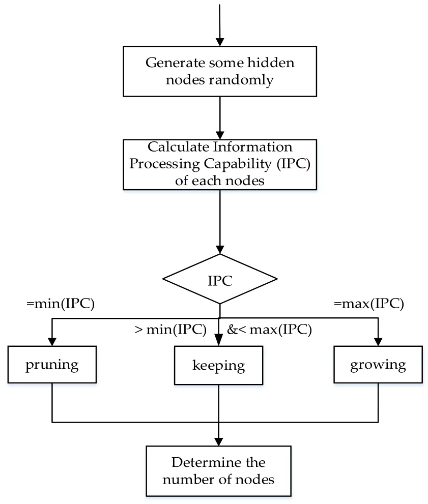
Figure 3:Logical scheme of the growing and pruning algorithm

The calculation of IPC is divided into two parts:the input IPC and output IPC,which are defined as:

x(t-K+1)is the input vector at time(t-K+1).The self-organizing algorithm contains three steps:growing step,pruning step and keeping step.The detailed process of each step is described below.

Growing Step.The largerandare,the information processing ability of the node is more powerful.In this case,if the IPC satisfies the following conditions:

Pruning Step.Like the above step,if the IPC of a node satisfies the following conditions:

If the input IPC vector of a node is the minimum value among all input IPC vectors,and the output IPC vector is the minimum value among all output IPC vectors,the node will be removed.The connection weights of neighbor nodes will be adjusted.

Keeping Step.If the input IPC as well as output IPC of a hidden node is not equal to the maximum information processing capability(such as Eq.(9))or the minimum information strength(such as Eq.(10)),the node will be kept.

2.4 The improved LSTM.

The number of hidden nodes is really important because it can directly affect the performance of the neural network.In more detail,if the number of hidden nodes is too small,the learning ability of this network will be weak.Even if the network is able to learn,it will cost a lot of time to train and the training accuracy is very likely to be low.When the number of neurons in the hidden layer is in a reasonable range,increasing the number of neurons can improve the precision of the network training,and may also reduce the number of training.But when it goes beyond that,if the number of neurons is continuing to be increased,the time for network training increases,and it may even cause other problems.So selecting a suitable number of hidden nodes is a vital problem which is difficult to handle.In order to solve this problem,an improved LSTM is proposed.And the flowchart of this work is displayed in Fig.4.

Figure 4:Flowchart of this research work

First,at the data preprocessing stage,a method called mutual information is used to select some features,which have a significant impact on PM2.5concentration.Second,these features are as input data for LSTM neural network.During the training period,a selforganizing algorithm called growing and pruning method is adopted to decide the most suitable number of nodes of the hidden layer.Finally,after training and testing,the result,that is,the predicting PM2.5concentration is as output of the neural network.

3 Experiment

In order to predict the concentration of PM2.5comprehensively and accurately,not only the hourly precise prediction but also the daily longer-term prediction is taken into account.

3.1 Data preprocessing

To predict PM2.5concentration,this study uses hourly and daily files of Nanjing,which include meteorological data as well as air pollutants.The meteorological data were collected from Meteorological Data Center of China Meteorological Administration,and the data sources of air pollutants were from Environmental Monitoring Stations of China.The meteorological data and pollution data were collected from the same stations,namely,Maigao Bridge,Caochang Gate,Shanxi Road,Zhonghua Gate,Ruijin Road,Xuanwu Lake,Pukou,Olympic Sports Center and Xianlin University City.Then data were averaged before experiment.Fig.5 displays a map of the location of each station.

Figure 5:Distribution of stations

These nine stations are distributed in all districts of Nanjing,so the average value well reflects the overall PM2.5level of Nanjing.

3.1.1 Singular value and missing value processing

There are 2664 records in the hourly dataset,and the time interval for the volume of data is one hour.And there are 1320 records in the daily dataset,where the range is from May 13thin 2014 to December 31stin 2017,and each value is the average value of a day.Raw data contains 27 factors,such as O3,NO2,CO,SO2,pressure,relative humidity,temperature and so on.These meteorological data and pollutant data do not change smoothly,but randomly.However,in the process of recording and calculating,there are some error values(like “937772(μg/m3)”).Also there are some missing values.these values will affect the performance of prediction.In order to avoid this problem,this paper uses the average values of neighbor data to replace these values.

3.1.2 Feature selection

Then,after the standardization,in order to select the main factors with respect to PM2.5concentration,a selection method called Mutual Information(MI)is adopted.Claude Shannon,a famous mathematician,pioneered the information theory in the middle of the 20th century and put forward a key concept-entropy,which is used to measure the uncertainty of a given probability distribution.MI is a method in information theory.It mainly calculates how much influence one thing has on the appearance of another.It is a measurement method for calculating how much information one attribute feature contains another attribute feature.The formula of mutual information is as follows

p(x,y)is the joint distribution of two characteristic variables x and y,andp(x)andp(y)represent the marginal distribution of two characteristic variables respectively.

This method can calculate that whether there is a relationship between the two variablesXandY,as well as the strength of the relationship.As a result,the MI values of these factors are high:O3,NO2,PM2.5,pressure,windy speed of instant maximum,wind direction of instant maximum,temperature,wind direction of maximum wind speed,relative humidity,water vapor pressure,minimum relative humidity,horizontal visibility,and body temperature.

3.2 Verification and validation

Through Section 3.1.2,several features were selected by a feature selection method.These features are as input data for LSTM neural network,which are O3,NO2,PM2.5,pressure,windy speed of instant maximum,wind direction of instant maximum,temperature,wind direction of maximum wind speed,relative humidity,water vapor pressure,minimum relative humidity,horizontal visibility,and body temperature.Learning rate is set to be 0.1,loss function is Mean Absolute Error(MAE).

mis the number of samples,yis the monitoring value andis the predicted value.

3.2.1 Hourly prediction

For hourly prediction,the model is fit for 500 training epochs,the dataset is splitted into training,validating and testing sets,training set is set to be 2000 records,validating set is set to be 563 and tesing set is set to be 100 records.

To prove that the number of hidden nodes decided by the self-organizing algorithm is the most suitable one,some different numbers of hidden nodes are used for comparison.Tab.1 shows the result of predicting PM2.5concentration after 1 hours,4 hours,8 hours and 12 hours.

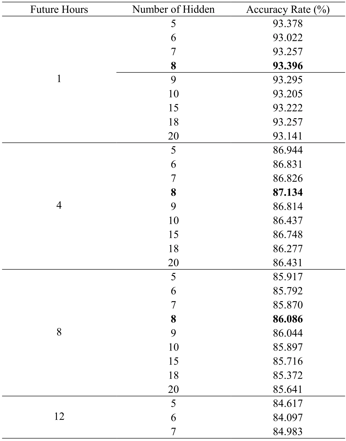
Table 1:The hourly predicting comparison between different numbers of hidden nodes

8 85.916 9 84.979 10 85.037 15 85.082 18 84.793 20 84.985

According to the self-organizing algorithm,the number of hidden nodes is determined to be 8.From Tab.1,when prediction interval time is set to be 1 hour,4 hours,8 hours and 12 hours,the correlation rates of 8 hidden nodes are the highest when compared with other number of hidden nodes.So the self-organizing algorithm is proved to be effective.Also,according to this table,the longer the prediction interval is,the lower the accuracy of the prediction will be.

In order to validate the superiority of the SSHL-LSTMNN for hourly prediction,there is a comparison experiment between the SSHL-LSTMNN and other neural networks.From the perspective of network structure,this paper adopts extreme learning machine(ELM),which is a kind of feedforward neural network and recurrent neural network(RNN),which contains a self-feedback structure,to compare with the neural network which is proposed by this paper.In addition,the Self-organizing Single Hidden-Layer ELM(SSHL-ELM)and the Self-organizing Single Hidden-Layer RNN(SSHL-RNN)are used as the comparison benchmarks as well.This experimrnt adopts these models to predict PM2.5concentration of next 1 hour,4 hours,8 hours and 12 hours in Nanjing.In Fig.5,the X-axis is the quantity of the testing samples,and the Y-axis is the absolute Difference-value(D-values)between measured data and predicted data of different models.Red line represents SSHL-LSTM,blue line represents ELM,green line represents RNN,black line represents SSHL-ELM and purple line represents SSHL-RNN.

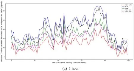
Figure 6:Absolute D-values between measured data and predicted data of different models for the testing dataset for one-,four-,eight-,and twelve-hour

From Fig.6,it can be observed that the red line is always the lowest,which means the absolute D-values between measured data and predicted data of SSHL-LSTM are the smallest.So the prediction accuarcy of SSHL-LSTM is proved to be the highest.Though sometimes the curves overlap partially because the predicted values are close,on the whole,the order of prediction accuracy from high to low is:SSHL-LSTM,SSHL-RNN,RNN,SSHL-ELM and ELM.As the time interval lengthens,the prediction accuarcy of each model is getting lower.Tab.2 describes the average predicting correlation rates between different models.

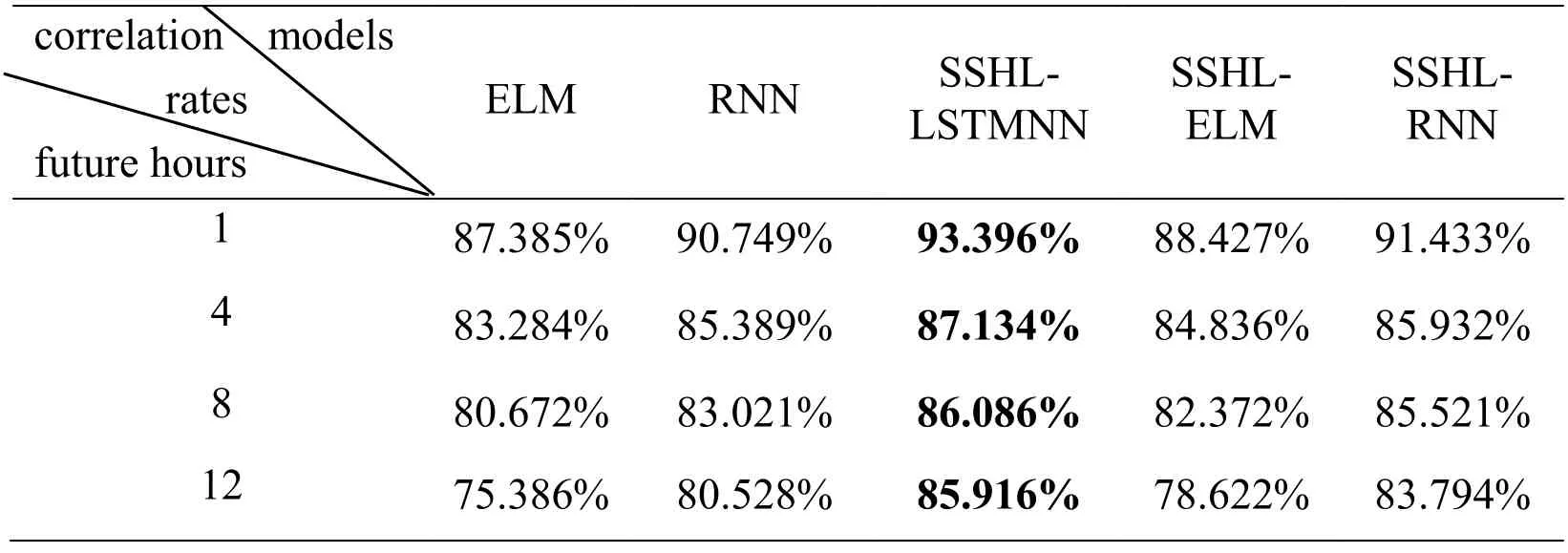
Table 2:The hourly predicting comparison between different models

According Tab.2,the correlation rates of different neural network for PM2.5prediction are displayed.Obviously,SSHL-LSTMNN algorithm shows higher correlation rates than ELM,RNN,SSHL-ELM and SSHL-RNN regardless of the time interval.Also,the prediction accuarcy of SSHL-ELM is higher than that of ELM,and SSHL-RNN is higher than RNN.So the self-organizing algorithm is proved to be effective.From the perspective of network structure,ELM is a kind of feed-forward neural network,which has no feedback loop in the network,so it cannot combine values of history moment as input.But the meteorological data and pollutant data this paper used are typical time series data,which means there is a strong correlation between the trend of data and time.So feed-forward neural network is not able to show a good capability for PM2.5prediction.Unlike ELM,RNN has feedback loop in its structure.So RNN can store the history data for the future prediction.However,because of the method of weight updating,RNN can't perform well for long-term prediction.So LSTM neural network is proposed for solving this problem.Therefore,LSTM neural network has better capability than feed-forward neural network and recurrent neural network.

3.2.2 Daily prediction

For daily prediction,input data are the same as those of hourly prediction.Learning rate is set to be 0.1,loss function is MAE.The model is fit for 300 training epochs,the dataset is splitted into training,validating and testing sets,training set is set to be 1000 records,validating set is set to be 220 and tesing set is set to be 100 records.

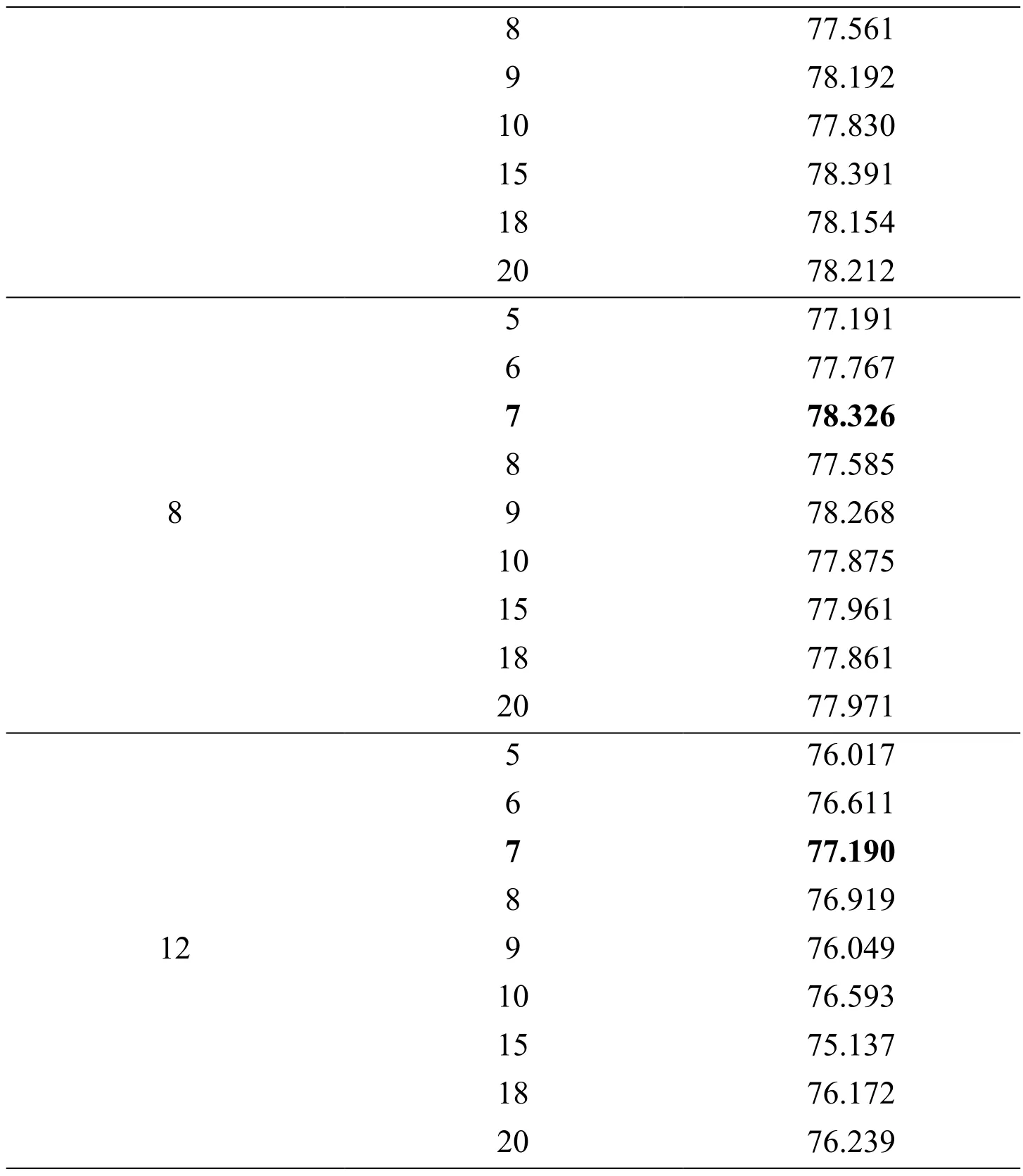
Hourly prediction can forecast near-time concentration of PM2.5instead of daily average concentration.So this section uses daily dataset to evaluate the daily prediction performance.After training by the self-organizing algorithm,the number of hidden neurons is set to be 7.To validate this result,a comparison experiment is operated.The results are shown in Tab.3.

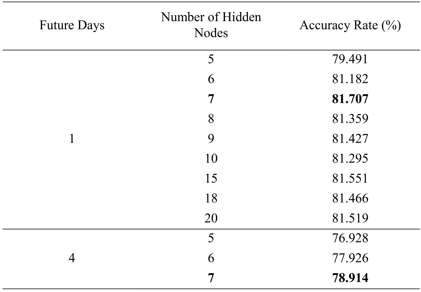
Table 3:The daily predicting comparison between different numbers of hidden nodes

8 77.561 9 78.192 10 77.830 15 78.391 18 78.154 20 78.212 5 77.191 6 77.767 7 78.326 8 77.585 8 9 78.268 10 77.875 15 77.961 18 77.861 20 77.971 5 76.017 6 76.611 7 77.190 8 76.919 129 76.049 10 76.593 15 75.137 18 76.172 20 76.239

According to the self-organizing algorithm,the number of hidden nodes is adjusted to be 7.From Tab.3,it is obvious that when the number of hidden nodes is 7,correlation rates perform better than other conditions.So the self-organizing LSTM model is proved to be effective.However,comparing with Tab.1,the prediction accuracy of daily prediction is much lower than hourly prediction.So this method is more applicable for short-term forecasting.

In order to validate the outstanding performance of the proposed model,Fig.7 shows the displays the curves of the absolute D-values between measured data and predicted data of different models.

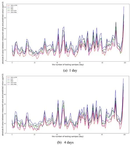
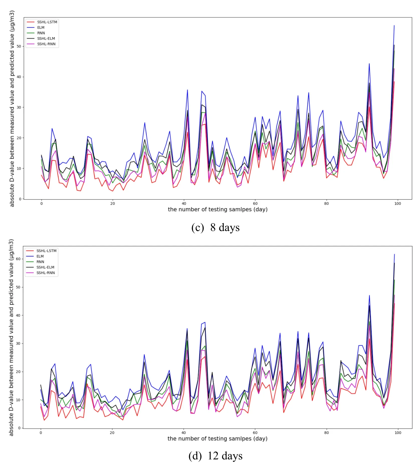
Figure 7:Actual and predict PM2.5 concentration for the evaluation dataset for one-,four-,eight-,and twelve-day

From Fig.7,it can be seen that the red line is always the lowest,which means the absolute D-values between measured data and predicted data of SSHL-LSTM are the smallest.So the daily prediction accuarcy of SSHL-LSTM is proved to be the highest.Compared to hourly prediction,the clearance of curves of different models is smaller,which means the daily prediction accuarcy is closer between different models.

Tab.4 describes the average predicting correlation rates between different models.

Table 4:The daily predicting comparison between different neural networks

According to Tab.4,SSHL-LSTMNN also performs best for daily prediction.But compared with Tab.2,the correlation rates are much lower than hourly prediction.In addition,the changes of correlation rates are not very significant when time interval changes.It may because the correlation between daily data is not as strong as that between hourly data,so it's difficult to fit the nonlinear relationship between daily data.

5 Conclusion and future work

Because meteorological data and pollutant data are typical time series data,LSTM network is suitable to apply in this case for its memory capability.Therefore,this paper proposed a machine learning method,an improved LSTM neural network to predict hourly and daily PM2.5concentration.The improved LSTM neural network was trained by a self-organizing algorithm,which solved the problem that the number of hidden layer nodes was difficult to determine.Experimental results verified the superiority of the SSHL-LSTMNN algorithm.

For future work,topographic condition and weather condition should be taken into account.For example,Nanjing is surrounded by mountains on three sides,the terrain is typical “dustpan” shape.It is easy to form unfavorable meteorological conditions such as static wind and inversion temperature.The diffusion conditions of atmospheric pollutants are poor.Especially in autumn and winter,it is easy to have continuous and steady foggy weather,which leads to moderate and severe pollution.More different topographic conditions like plateau and Plain can be researched in the future.

Acknowledgement:This work was supported by Scientific Research Project of The Education Department of Hunan Province(Grant No.17C0479)and Marie Curie Fellowship(701697-CAR-MSCA-IF-EF-ST).