OPTIMAL DIVIDEND AND FINANCING PROBLEMS FOR A DIFFUSION MODEL WITH EXCESS-OF-LOSS REINSURANCE STRATEGY AND TERMINAL VALUE

LI Tong,MA Shi-xia,Han Mi

(School of Sciences,Hebei University of Technology,Tianjin 300401,China)

Abstract:In this paper,we investigate the optimal dividend and financing policies problems with excess-of-loss reinsurance and a terminal value.In our model,by using approximate diffusion and dynamic programming and constructing of suboptimal problems,we obtain the HJB equation satisfied the general optimal problem and verification theorem.Assuming the proportional and fixed transaction costs and the terminal value at bankruptcy,we get the optimal value function,the optimal dividend policy,the optimal reinsurance strategy and the optimal finance strategy.

Keywords: diffusion process;dividend and financing;excess-of-loss reinsurance;expected value principle;terminal value

1 Introduction

In the actuarial and mathematical insurance literature,the optimal dividend problem for an insurance company consists in finding a dividend strategy that maximizes the expected discounted dividends until the ruin.The diffusion model about this problem of optimal risk control and dividend distribution was widely studied since fifteen years ago.As we know,the diffusion models for companies can control risk exposure and dividend payment.For example,the papers such as Taksar and Zhou[1],Asmussen et al.[2]and Cadenillas et al.[3]considered that the company control the risk exposure by proportional reinsurance.Meanwhile,some increasing attention was paid to the dividend problem in term of excess-of loss reinsurance.The literature includes Zhang and Zhou[4],Xu and Zhou[5]and reference therein.

When companies are on the verge of ruin,we can choose to bail out through capital injections or get out of business.When the surplus is null,we inject to prevent bankruptcy,see He and Liang[6]and Peng and Chen[7].Leaving the business may lead to bankruptcy and the corresponding terminal value(say P).For P≥0,we view the terminal value as salvage value;for P<0,it is viewed as the penalty value.The terminal value considered by the optimal control problem goes back to Karatzas et al.[8].Taskar[9] firstly considers the risk control and dividend distribution problem with terminal value.Since then,more and more attention are paid on the control problem with terminal value.For instance,the optimal proportion reinsurance policy with terminal value can be found on Taskar[9].Albrecher[10]and Liang and Young[11]found the optimal dividend strategy in diffusion risk model under a penalty(or salvage)for ruin.Some papers consider the optimal dividend and financing strategies with terminal value and reinsurance polices under different premium principle.For example,Yao and Yang[12]and Cheng and Zhao[13]investigated the optimal problem under the variance premium principle.Cheng and Wang[14]solved this problem under the exponential premium principle.Considering the excess-of-loss reinsurance,Xu and Zhou[5]and Liu and Hu[15]started to research on this optimal problem.As far as we know,very little work has considered the combined optimal dividend,excess-of-loss reinsurance and financing polices with terminal value.

Motivated by the above references,in this paper we study the optimal dividend, financing and excess-of-loss reinsurance with terminal value.The paper is organized as follows.In Section 2,we introduce the model formulation of the problem.In Section 3,we give the HJB equations about the optimisation problem and some properties of the value function.In Section 4,we consider the optimal control problem without capital injection.In Section 5,we solve the optimal problem that the company does not allow to ruin through financing.

2 Model Formulation and the Optimal Control Problem

Let(Ω,F,{Ft}t≥0,P)be a probability space,on which all stochastic quantities in this paper are well defined.Here{Ft}t≥0is a filtration,which satisfies the usual conditions.To specify the diffusion model, firstly,we introduce the classical Cramer-Lundberg risk model.The surplus process of an insurance company satisfies

where Z0=x ≥ 0 is the initial reserve and c≥ 0 is the premium rate.{Nt}t≥0is a Poisson process with constant intensity λ.Yiis the size of the ith claim,where Yiare independent and identically distribution positive random variables with common distribution function F.Assume that mean µ1=E[Yi]>0 and the second momentµ2=E[Yi2]>0 are finite.

In this paper,excess-of-loss reinsurance is available,so let a be the excess-of-loss retention level.Assume the insurer purchases reinsurance contract R to cede the risk of claim,that is to say,the insurer covers R(Yi)for claim Yi,and R(Yi)=Yi∧a.Then define the correspondingandThe premium rate for the reinsurance covers cR,under the expected value principle,it haswhere θ is the safety loading,and

By the same argument as in the Asmussen et al.[2],we can approximate the process(2.3)by a pure diffusion process{}with the same coefficient and volatility.Specifically,{}satisfies

where{Bt}is a standard Brownian motion,adapted to the filtration{Ft}.Assume the retention level can be dynamically adjusted to control the risk expose.At each time,the insurer chooses the retention level a=a(t).

Next,we consider dividend payment and capital injection in the above processes.Denote Ltas the cumulative amount of dividends paid up to time t.The capital injection processis described by a sequence of random variables{ηn,n=1,2,···}and a sequence of increasing stopping times{τn,n=1,2,···},which are corresponded to the amounts of capital injections and the times,respectively.Then given an admissible control strategy π =(aπ,Lπ,Gπ),the dynamics of the control surplus process{}with initial reserve x>0 can be written by

In this paper,using the excess-of-loss reinsurance strategy means that among the admissible reinsurance policies the retention level{at}can be adjusted dynamically to reach the whole optimization.In addition,we assume that the insure company premium under expected premium principle is c=(1+θ)λµ(1),which is the case of cheap reinsurance.Thus,the process{}can be written as the following stochastic process

Then we give the following definition of an admissible strategy which the insurer can select.

Definition 2.1 A strategy π is said to be admissible if

Condition(ii)implies the reserve available is more than the total amount of dividends at the moment.Condition(v)demands that the capital injections may not occur in finitely in a finite interval.Denote by Π the set of these admissible strategies.For each admissible policies π∈Π,the ruin time of the control surplus process is defined as Tπ=inf{t≥0:<0},which is first time that surplus becomes negative.Then we can study the following problem.

We measure the company’s value associated with strategy π ∈ Π using the following performance function V(x;π),which is the expected sum of discounted terminal value and the discounted dividends less the expected discounted costs of refinancing until the time of ruin

Exdenotes the expectation conditional on=x,and δ>0 is the discount rate.In the financing process,we assume that the shareholders need to pay β2η+K to meet the capital injection of η,where β2>1 measures the proportion costs,K>0 is the fixed costs.In the dividend distribution process,proportion costs transaction are taken into account through the value β1,β1∈ (0,1)means that the shares can get β1l if the company pays l as dividends.

The objection is to find the optimal value function

and the associated optimal strategy π∗such that V(x)=V(x;π∗).

3 The Hamilton-Jacobi-Bellman(HJB)Equation and Verification Theorem

The solution of the optimal value function and the optimal strategy are based on the HJB(Hamilton-Jacobl-Bellman)equation.In order to deriving this equation,we first define some operators.

For the function v(x):[0,∞)7→ R,we define the financing operator M by

which means the value of the police that consists of choosing the best immediate capital injection.The differential operator Aais denoted by

Assuming that the value function V(x)is the twice continuously differentiable,and using the standard stochastic control theory(see,e.g.,Fleming and Soner[16]),we can characterize the HJB equation of the control problem as

Then we will give some property of the value function.

Lemma 3.1 The value function defined by(2.8)is increasing on[0,∞)with

and satisfies the following boundary condition

Proof Given ε ≥ 0,take a admissible strategy π1∈ Π such that V(x;π1)≥ V(x)− ε.For each x ≥ y ≥ 0,we define a new strategyeπ1∈ Π as follows:issue equities with the amount of x − y and then follow the strategy π1.The strategy π1is admissible and we have

ε is arbitrary.So we obtain the second inequality.The first inequality can be similarly proved.

Consider a new strategy π2.When we pay all of the surplus as dividends and claim the terminal value,we can get the corresponding performance function V(x;π2)= β1x+P.Because of the optimality of the value function,we obtain V(x)≥ V(x;π2)= β1x+P.

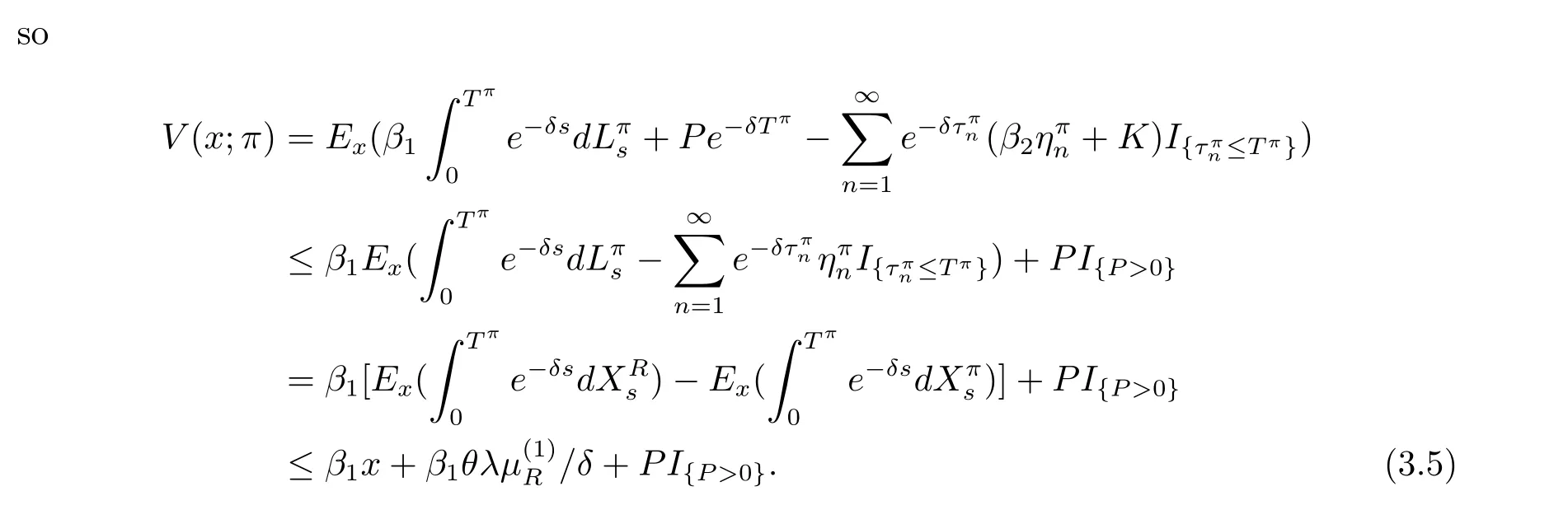
Hence,we can get the boundary condition.

Theorem 3.1(Verification theorem)Let v(x)be a twice continuously differentiable,increasing and concave solution of HJB equations(3.1)and(3.2),and v0(x)is bounded,then for each π ∈ Π,we have v(x)≥ V(x;π).So v(x)≥ V(x)for all x ≥ 0.Moreover,if there exists some strategy π∗=(aπ∗,Lπ∗,Gπ∗)such that v(x)=V(x;π∗),then v(x)=V(x)and π∗is optimal.

Proof For each given strategy π =(aπ,Lπ,Gπ) ∈ Π,let’s define={s:6=be the discontinuous part ofand=−be the continuous part of.Similarly,andstand for the discontinuous and continuous parts of,respectively.Then,using Itˆo’s formula,we have

The sum of discontinuous parts of last term can be written as

where the inequality holds,because v(x)satisfies the HJB(3.1)with v0(x)≥ β1and Mv(x)≤v(x).Moreover,in consideration of(3.1),the first term of the right hand side of(3.6)is

non-positive.Therefore,by substituting(3.7)into(3.6),we have

Because v(x)is an increasing function and v(0)≥P,we obtain

Taking expectation and limitation on both sides yields

Consequently,v(x)≥V(x)follows.

4 The Case without Capital Injection

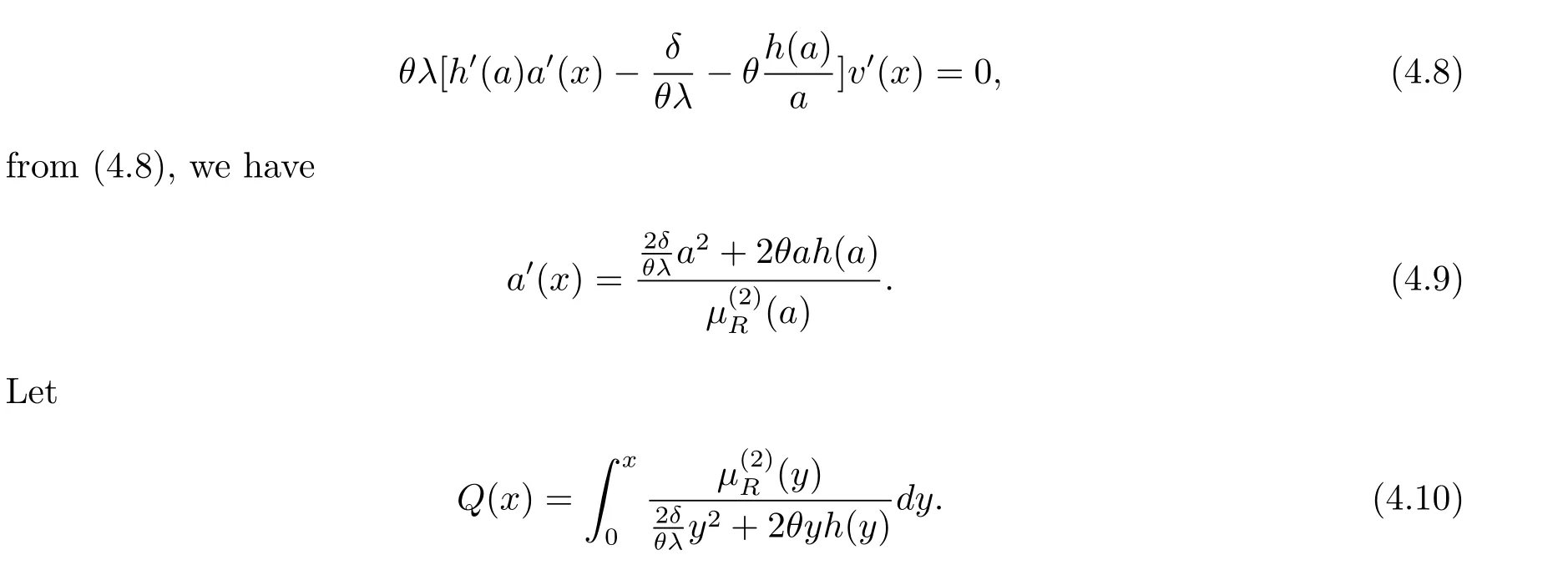
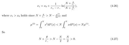
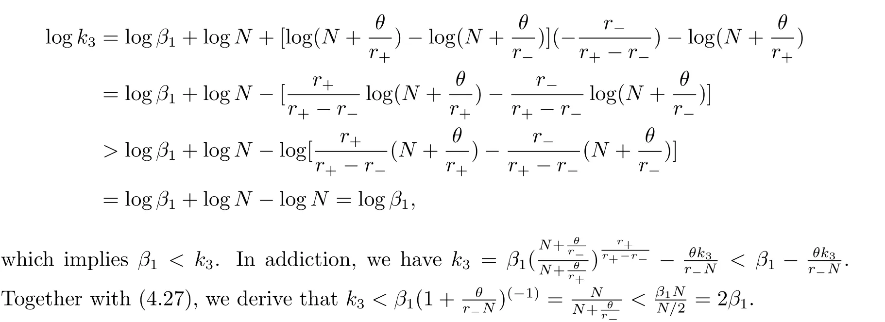
In this section,we consider the first case when the policy without capital injection is optimal.Hence,the corresponding boundary condition is v(0)=P and Mv(0)≤v(0).Let x1=inf{x;v0(x)=β1}.Then,the solution v(x)satisfies the following equations

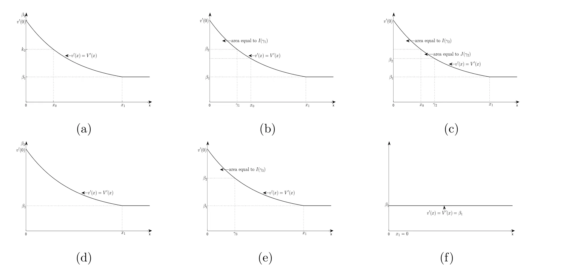
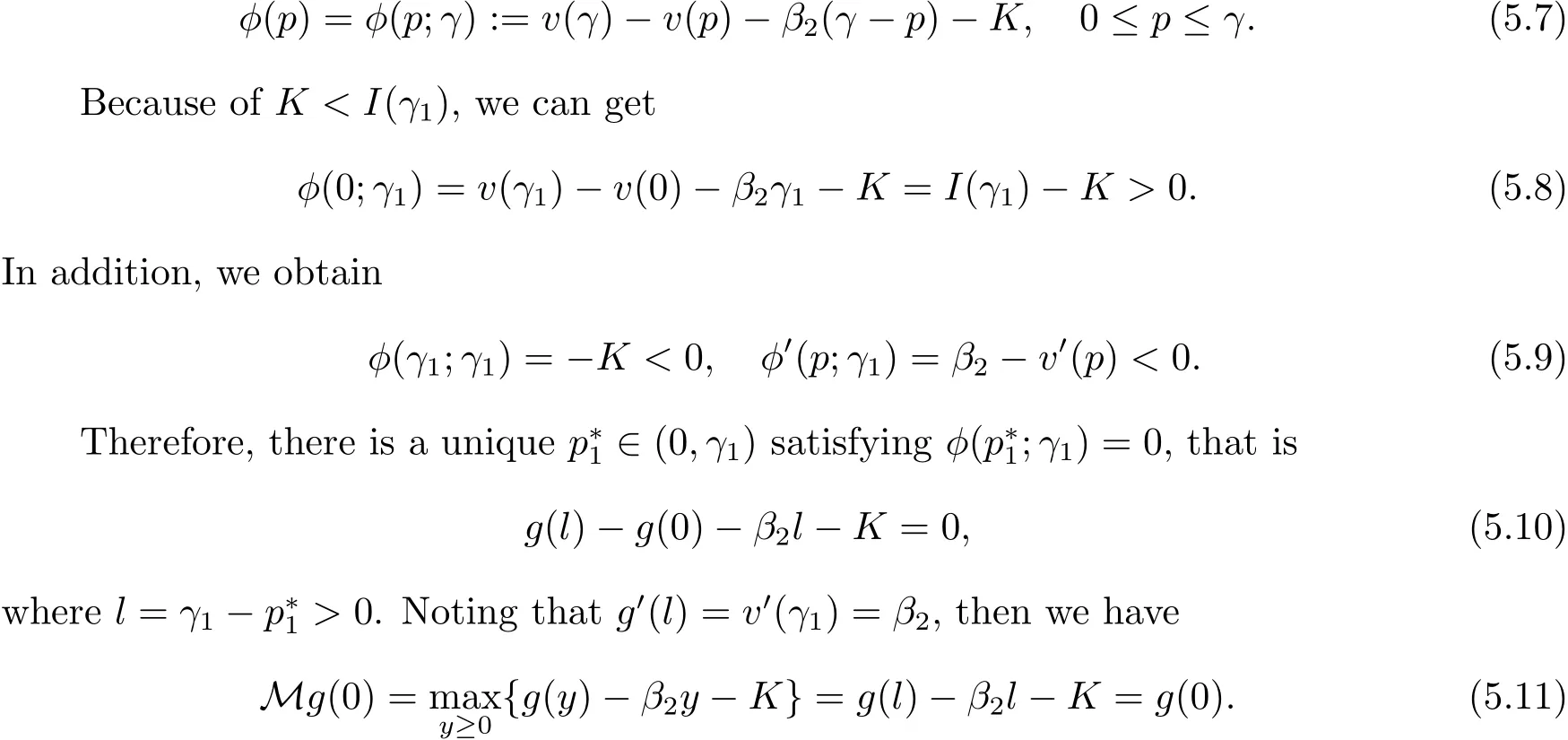
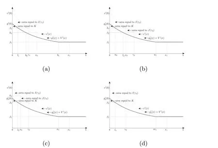
In fact,these equations indicate that the continuous region is(0,x1),and the dividend region is[x1,∞).For 0 ≤ x

then let the derivative equal to zero yields

In view of(2.2),the maximizer of the left-side of(4.1)satisfies the above equation.Substituting(4.6)into(4.1)leads to

It is easy to obtain that Q0(x)≥0,so the inverse function of Q(x)exists,we have

There exists some constant k such that

Since a0(x)≥0,the a(x)is a strictly increasing function.Next,we suppose that there exists a reinsurance level x0is smaller than that for dividend x1,that is,the insurer will keep all the claims when the surplus exceeds x0,and we have Q(N)=x0+k.Thus,from(4.12),we get

For 0≤x

where k3is unknown coefficient.

Meanwhile,for x0≤x

Then the solution of(4.15)is of the form

where k1and k2need to be determined,and

Thus,the solution of HJB equation is

According to the principle of smooth fit and calculating the first and the second derivatives of v(x)at x0and x1,respectively,we have

Solving(4.20)and(4.21)leads to

Meanwhile,by multiplying(4.22)by−and subtracting it from(4.23)yields

Thus,we can obtain

Using(4.22)and(4.24),we get

Lemma 4.1 β1

Proof According to the concavity of the log function,we get

Next,we come to determine the value a(0),x0and x1.For 0≤x

From(4.13)and(4.26),we can know once the a(0)is determined,the value of x0and x1can be calculated.In view of(4.14),we have

Then,together with the(4.29),we obtain

Let’s apply a variable change of y=a(s)and use(4.9)and a(x0)=N,we get

where the function of g(x)is written as g(x)x>0.After some simple calculations,it is easy to know that g(0+)=0,g(N)=h(N)= µ(1)−,andThen we obtain that the g(x)is a strictly increasing function on[0,N].Thus we can get that(4.32)determines a unique root a(0)on[0,N]if the conditionholds.Thus,we will confirm(4.4)in the following cases.

(1)If P ≤θwe are aware of v0(x)is decreasing on[0,∞),so v0(x)≤ β2holds for x≥ 0.Thus Mv(0)−v(0)=(4.4)holds.In this case Figure 1(a)is a graph of v0(x).

Obviously,(4.4)is valid if and only if when K ≥ I(γ1).In this case Figure 1(b)gives a graph of v0(x).

we know J(γ2)is decreasing with regard to β2.(4.4)holds if and only if when K ≥ J(γ2).

Figure 1:The graph of the derivative v0(x)=V0(x).

In this case,Figure 1(c)provides a graph of v0(x).there is no solution to solve(4.32).In this case,it shows that there does not exist x0>0 such that a(x)

If P>

According to the principle of smooth fit at x=x1and the boundary condition v(0)=P,we have

In order to prove the existence of x1,we define ϕ(x)=k1e−r+x+k2e−r−x.We find thatand ϕ(∞)= −∞.Therefore,whenholds,(4.37)will have a unique root of x1>0.

(4.4)holds.In this case,Figure 1(d)is a graph of v0(x).

5 The Case with Capital Injection

In this section,we consider the case with capital injection,namely,it is optimal to inject capital to prevent bankruptcy only when the surplus is null.Thus,the solution of g(x)should satisfy

where b1≥ 0 is the level of the dividend policy.Similar to Section 4,we solve(5.1)–(5.2)as the following cases.

where b0=x0− p∗1,b1=x1− p∗1;x0,x1and v(x)are written by(4.13),(4.26)and(4.19),respectively.Correspondingly,we define the optimal reinsurance strategy by

Denote

Thus,(5.1)–(5.4)hold.In this case,Figure 2(a)is a graph of v0(x)=g0(x).

Figure 2:The graph of the derivative g0(x)=V0(x).

where u0=x0−>0,u1=x1−>0 and∈ (0,x0)is the unique solution to φ(p;γ2)=0,i.e.,

where l2= γ2− p∗2>0.Meanwhile,define a optimal reinsurance policy by

Thus,(5.1)–(5.4)hold.In this case,Figure 2(b)gives a graph of v0(x)=(x).

where n1=x1−>0,and∈ [x0,γ2)is the unique solution to φ(p;γ2)=0,i.e.,

where l3= γ2−>0.The optimal reinsurance strategy is(x)≡ N.Thus,(5.1)–(5.4)hold.In this case,Figure 2(c)is a graph of v0(x)=(x).

where m1=x1−>0,and∈ (0,γ3)is the unique solution to φ(p;γ3)=0,i.e.,

where l4= γ3− p∗4>0.The optimal reinsurance strategy is(x)≡ N.Thus,(5.1)–(5.4)hold.In this case,Figure 2(d)provides a graph of v0(x)=(x).

Based on the above analysis,we identify the explicit solution to the value function and construct the associated optimal strategy in the following.In order to the following theorem,let

Theorem 5.1 The value function V(x)and the corresponding optimal reinsurance policy π∗=(aπ∗,Lπ∗,Gπ∗)are given in the following different cases.

by(5.14).

Proof Here we only prove Case 7 in detail as an example and the other cases also can be proved by this method.By verifying the second derivative of g(x),we can check the concavity of g(x)function.For 0≤x

For b0≤x

In addition,we can prove that the value function g(x)is indeed an increasing,concave and twice continuously differentiable solution to equations(3.1)and(3.2).Using Theorem 3.1,we can show that the solution to HJB eq.(3.1)and(3.2)exactly equal to the value function.Thus,g(x)≥V(x)holds according to Theorem 3.1.Here we omit the details when g(x)satisfies(3.1)and(3.2).Then,from(5.6),(5.19)and(5.21)we will check the optimal policy π∗=(aπ∗,Lπ∗,Gπ∗) ∈ Π,where u=b1in(5.19).Because offor 0≤≤b1,it follows

Meanwhile,(5.6),(5.19)and(5.21)indicate that

Thus,from(3.6),substituting π,Tπ,u with π∗,Tπ∗= ∞,b1and taking expectations,we get

Let t→∞,the first term on the right hand side vanishes,therefore,we have

considering g(x)≥ V(x),we check that g(x)=V(x)=V(x;π∗).