WEIGHTED MIXED INEQUALITIES ON PRODUCT SPACES WITH MUCKENHOUPT BASES

CHEN Wei,ZHU Chun-xiang,ZHANG Chao

(1.School of Mathematical Sciences,Yangzhou University,Yangzhou 225002,China)

(2.School of Statistics and Mathematics,Zhejiang Gongshang University,Hangzhou 310018,China)

Abstract:We study weighted mixed inequalities on product spaces with different Muckenhoupt bases.Our approaches are mainly based on the abstract formalism of families of extrapolation pairs and Minkowski’s integral inequality.Moreover,we can deduce the general case of our results by induction.

Keywords:mixed norm Lebesgue space;Muckenhoupt basis;extrapolation

1 Introduction and Statements of Main Results

In this paper,we shall deal with spaces of measurable functions defined in the following way.Let(Xi,Si,µi),for 1 ≤ i ≤ n,be totally σ- finite measure spaces and P=(p1,p2,···,pn)a given n-tuple with 1 ≤ pi≤ ∞.We always suppose that none of the spaces(Xi,Si,µi)admits as the only measurable functions the constant ones.A function f(x1,x2,···,xn)measurable in the product space,is said to belong to LP(X)if the number obtained after taking successively the p1norm in x1,the p2norm in x2,···,the pnnorm in xnand in that order,is finite.The number so obtained,finite or not,will be denoted by kfkP,kfk(p1,···,pn)or kfkp1,···,pn.When for every i,pi< ∞,we have in particular

If further,each piis equal to p:

and LP(X)=Lp(X)(see[1]for more information).In this paper,we only deal with the case when every component space(Xi,Si,µi)is a di-dimensional Euclidean space Rdiwith Lebesgue’s measure.Then,the product space(X,S,µ)is a d-dimensional Euclidean space with Lebesgue’s measure,where d=d1+d2+ ···+dn.

In the following,we consider weighted inequalities on these spaces.For simplicity of notations,we only consider the case of n=2 and our results can be extended to the general case by induction.

Throughout,ω will denote a weight,i.e.,a nonnegative,locally integrable function.All cubes in Rdiwill be half open with sides parallel to the axes.Given a set E⊂Rdi,|E|will denote the Lebesgue’s measure of E, ω(E)=(x)dx the weighted measure of E,andthe average of ω over E.

To define the classes of weights which we will consider,we first introduce the concept of basis B and the maximal operator MBdefined with respect toB(see[2,3]for more information).A basis B is a collection of open sets B ⊂ Rd.A weight ω is associated with the basis B,if ω(B)< ∞ for every B ∈ B.Given a basis B,the corresponding maximal operator is defined by

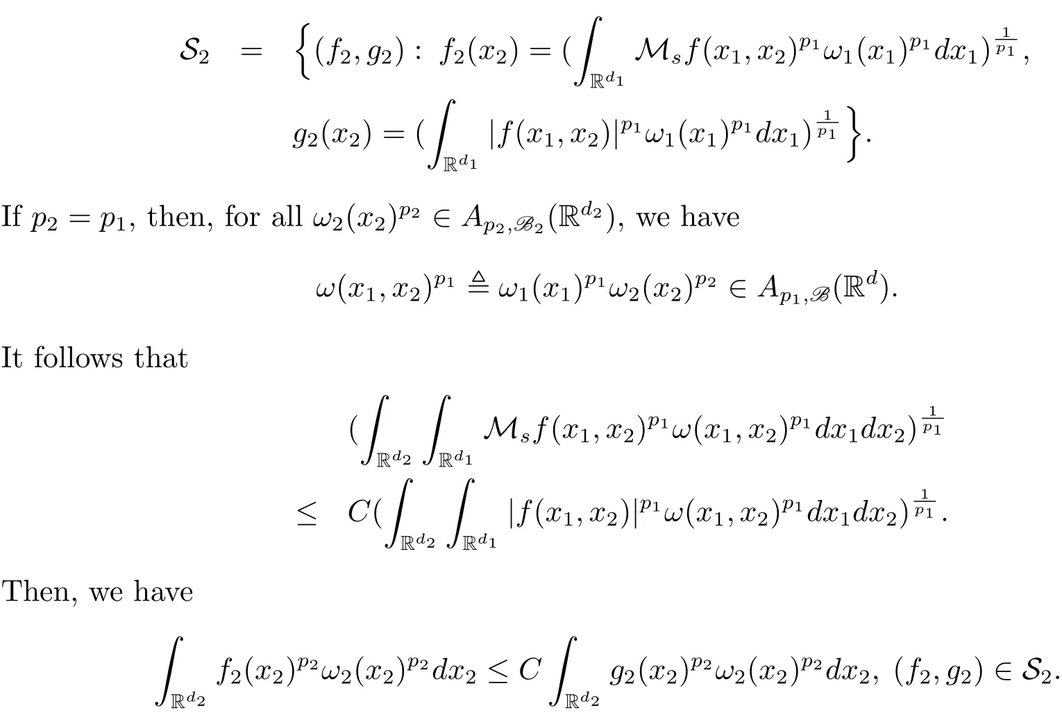
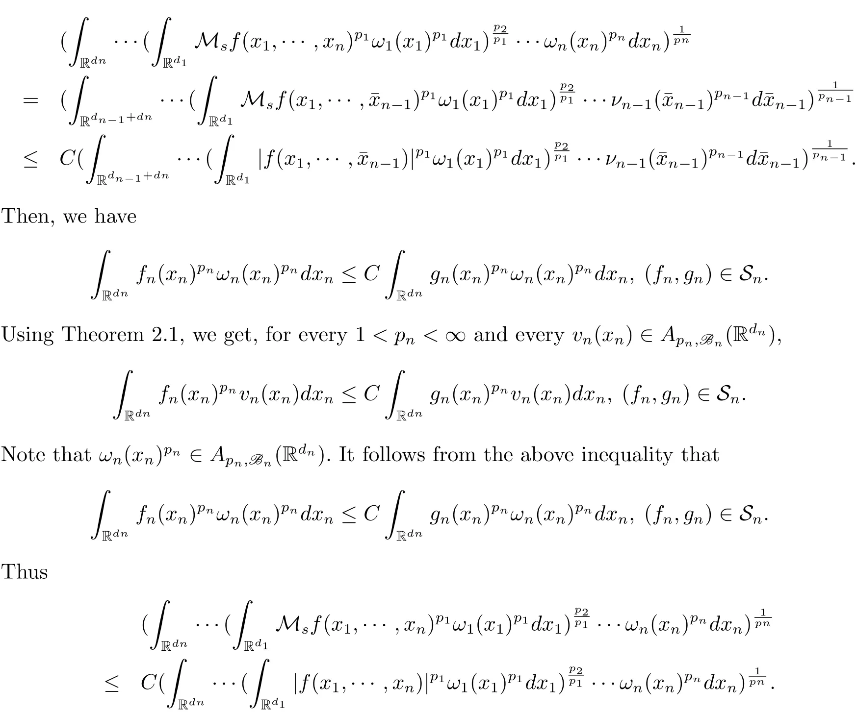
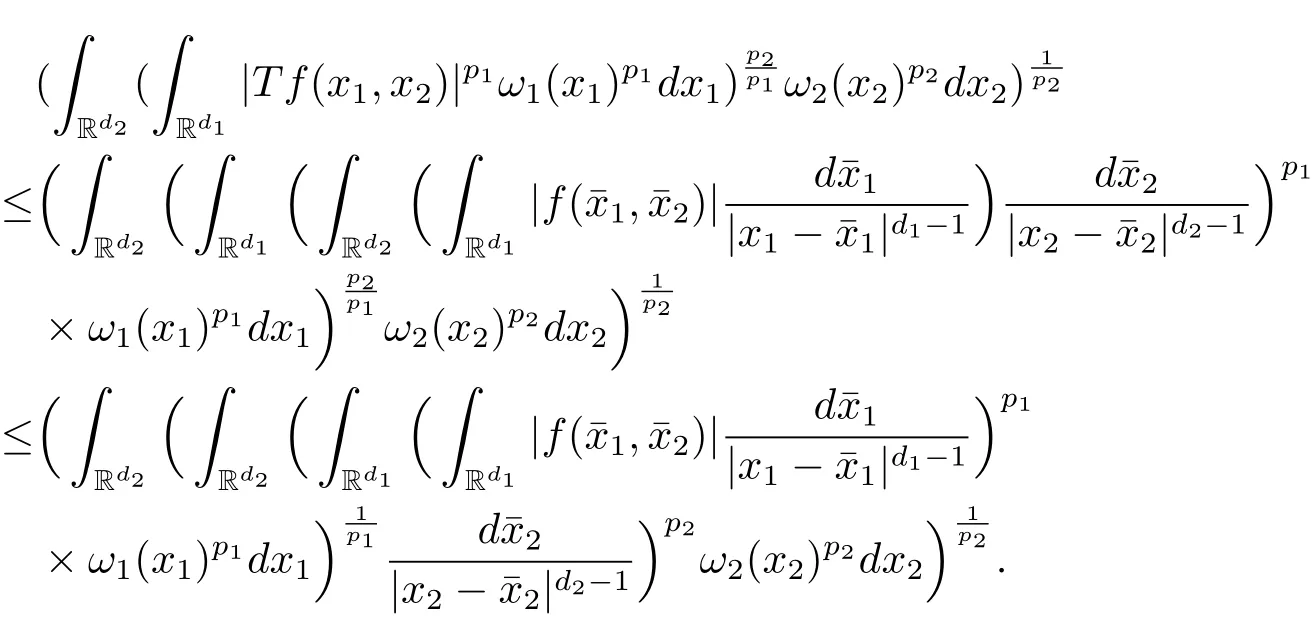
A weight ω associated with B is in the Muckenhoupt class Ap,B(Rd),1

When p=1,ω belongs to A1,B(Rd)if MBω(x)≤ Cω(x)for almost every x ∈ Rd.The infimum of all such C,denoted by[ω]Ap,B(Rd).For simplicity,Ap,B(Rd)is denoted by Ap,B,if no confusion can arise.Clearly,if 1≤q≤p,then Aq,B⊆Ap,B.Further,from the definitions we get the following factorization property:if ω1, ω2∈ A1,B,then ω1ω1−p2∈ Ap,B.Finally,we let

We are going to restrict our attention to the following class of bases.A basis B is a Muckenhoupt basis if for each p,1

Let B be a Muckenhoupt basis.Let 1

Muckenhoupt bases were introduced and characterized in[3,Theorem 2.1].Three immediate examples of Muckenhoupt bases are D,the set of dyadic cubes in Rd;C,the set of all cubes in Rdwhose sides are parallel to the coordinate axes,and R,the set of all rectangles(i.e.,parallelepipeds)in Rdwhose sides are parallel to the coordinate axes(see[4,Theorem 7.14]).One advantage of these bases is that by using them we avoid any direct appeal to the underlying geometry:the relevant properties are derived from(1.1),and we do not use covering lemmas of any sort.

In this paper,we will use the Rubio de Francia extrapolation as our main tool to deal with our inequalities.As is well known,the extrapolation theorem of Rubio de Francia is one of the deepest results in the study of weighted norm inequalities in harmonic analysis[5].Recently,an approach to extrapolation is based on the abstract formalism of families of extrapolation pairs and summarized by Cruz-Uribe[6].This approach was introduced in[7]and first fully developed in[8](see[9]for more information).It was implicit from the beginning that in extrapolating from an inequality of the form

the operator T and its properties(positive,linear,etc.)played no role in the proof.Instead,all that mattered was that there existed a pair of non-negative functions(|Tf|,|f|)that satisfied a given collection of norm inequalities.Therefore,the proof goes through working with any pair(f,g)of non-negative functions.

Hereafter,we will adopt the following conventions.A family of extrapolation pairs F will consist of pairs of non-negative,measurable functions(f,g)that are not equal to 0.Given such a family F,0

we mean that this inequality holds for all pairs(f,g)∈F such that kfkLp(w)<∞,i.e.,that the left-hand side of the inequality is finite and the constant C depends only upon p,q,d,and the[w]Aqconstant of w.Moreover,given a family F,0

The key to the new approach is the family of extrapolation pairs F.If the family of extrapolation pairs F seems abstract and mysterious,it may help to think of the particular family

where T and S are some operators that we are interested in and N is some “nice” family of functions:etc.We refer to Cruz-Uribe[6,Sections 5 and 6]and Cruz-Uribe,Martell and Pérez[9,Section 3.8]for more information.

Using the above conventions,we can give the following main results related with strong maximal operator,Riesz potential and multiparameter fractional integral operators.

Let B1and B2be Muckenhoupt bases in Rd1and Rd2,respectively.We consider the space Rd1×Rd2which identify with Rd1+d2=Rdand the product basis B,B1×B2={Qd1×Qd2:Qdi∈Bi}.The corresponding maximal operator is called strong maximal operator and is denoted by Ms.

Let 1

where ω(x1,x2)= ω1(x1)ω2(x2).Moreover,let B,C1× C2,it follows by Fubini’s theorem that B is a Muckenhoupt basis(see[8,Page 424]).

Then we have the following Theorem 1.1,which is a weighted version of[10,Theroerm 4.1].

Theorem 1.1 Let 1

(1)There is a constant C,independing of f such that

Let Rdbe the d-dimensional Euc1idean space.The Riesz potential of order α,0< α

We also define the fractional maximal operator M(α)f(x)by

where the supremum is over all cubes Qdwith sides parallel to the axes and containing x.

We extend[11,Theorem 1]to the case on mixed norm Lebesgue spaces.Let us consider the di-dimensional Euclidean space Rdiand the basis Ciin it,where i=1,2.For Rd=Rd1×Rd2,we consider two bases C and B=C1×C2in it.It is clear that C ⊆C1×C2.For C,Sjodin[12]obtained the following Theorem 1.2,which gave the weighted norm inequalities for Riesz potentials and fractional maximal functions in mixed norm Lebesgue spaces.We reprove the theorem by the abstract formalism of families of extrapolation pairs as following.

Theorem 1.2 Let 0

Also we can consider the fractional integral operators in our case.We define a multiparameter version of the fractional integral operator of order 1(see,e.g.[8,Page 423]):for(x1,x2)∈Rd1×Rd2,let

Given(x1,x2)∈Rd1×Rd2and a functiondefine the multi-parameter fractional maximal operators

A simple estimate shows thatand similarly with the order of composition reversed.As in the one-variable case,the reverse inequality does not hold pointwise,but does hold in the sense of weighted Lpnorms.For the product B,we have the following theorem,which is an extension of[8,Proposition 3.5].

Theorem 1.3 Let 1 ≤ p1< ∞,0

Throughout this paper,C denote a constant not necessarily the same at each occurrence.

2 Proof of Main Results

In this section,we give the proofs of Theorems 1.1–1.3.

To prove Theorem 1.1,we need the following theorem which was proved by Cruz-Urible,Martell and Pérez in[9].

Theorem 2.1 (see[6,Theorem 3.9])Given a family of extrapolation pairs F,let B be a Muckenhoupt basis.Suppose that for some p0,1≤p0<∞,and every w0∈Ap0,B,

Then for every p,1

Then,we can give the proof of Theorem 1.1 as follows.

Proof of Theorem 1.1 Suppose that(1.4)is valid.We proveand

We have Msf(x1,x2)=MB1h(x1)χQd2(x2).Then,we rewrite(1.4)as

It follows from(1.2)that ω1(x1)p1∈ Ap1,B1(Rd1).Similarly,we have

Conversely,to prove(1.4).Fix p1>1 and

Thus,we check(2.1)of Theorem 2.1 with F,S2and p0,p2.Using Theorem 2.1,we get,for every 1

Note that ω2(x2)p2∈ Ap2,B2(Rd2).It follows from the above inequality that

Kurtz[13]obtained Theorem 1.1 in the space Rd1×Rd2involving C1×C2and Theorem 1.1 is a general case of[13,Theorem 1].Here,it is natural to expect a more general result.

LetBibe a Muckenhoupt basis in Rdi,i=1,2,···,n.Thena product basis in the spaceis a Muckenhoupt basis in Rdi×Rdi+1,i=1,2,···,n − 1,using our approach to Theorem 1.1,we have the following Corollary 2.2 by induction.

Corollary 2.2 Let 1

(1)There is a constant C,independing of f such that

Proof We only prove(2)⇒(1)and this is done by induction beginning with the case n=2.For n=2,it is valid because of Theorem 1.1.

Assuming that the inequality is valid for n−1,we set

If pn=pn−1,then,for all ωn(xn)pn∈ Apn,Bn(Rdn),we have

It follows from the induction hypothesis that

This completes the induction step.

And therefore,we have the following remark.

Remark 2.3 LetBi=Ci,i=1,2,···,n,in the assumption of Corollary 2.2,then Ci× Ci+1is a Muckenhoupt basis in Rdi× Rdi+1,i=1,2,···,n − 1.

In order to prove Theorem 1.2,we need make some preparations.

It was well known that Muckenhoupt and Wheeden[11,Theorem 1]proved the following lemma.

Lemma 2.4 For every weight ω ∈A∞,C(Rd)and 0

Also,we need the following theorem proved in[9].

Theorem 2.5 Given a family of extrapolation pairs F,letBbe a Muckenhoupt basis.Suppose that for some p0,0

Then for every p,0

Then,we can prove Theorem 1.2 in the following.

Proof of Theorem 1.2 Fix 0

If p2=p1,then,for all ω2(x2)p2∈ A∞,C2(Rd2),we have

It follows from Lemma 2.4 that

Then,we have

Thus,we check(2.2)of Theorem 2.5 with F,S2and p0,p2.Using Theorem 2.5,we get,for every 0

Note that ω2(x2)p2∈ A∞,C2(Rd2).It follows from the above inequality that

At last,we give the proof of Theorem 1.3.First,we should remind that Cruz-Uribe,Martell and Pérez proved the following proposition in[8,Proposition 3.5],which is a special case of Theorem 1.3.

Proposition 2.6 [8,Proposition 3.5]For every weight ω ∈ A∞,C1×C2(Rd1×Rd2),

Now,we give the proof of Theorem 1.3 as follows.

Proof of Theorem 1.3 In view of the definition,we have

Using Minkowski’s integral inequality,we obtain that

Combining this estimate with Lemma 2.4,we have that

Using Lemma 2.4 again,we prove that