Fault Diagnosis of Motor in Frequency Domain Signal by Stacked De-noising Auto-encoder

Xiaoping Zhao, Jiaxin Wu, , Yonghong Zhang, Yunqing Shi and Lihua Wang

Abstract: With the rapid development of mechanical equipment, mechanical health monitoring field has entered the era of big data. Deep learning has made a great achievement in the processing of large data of image and speech due to the powerful modeling capabilities, this also brings influence to the mechanical fault diagnosis field.Therefore, according to the characteristics of motor vibration signals (nonstationary and difficult to deal with) and mechanical ‘big data’, combined with deep learning, a motor fault diagnosis method based on stacked de-noising auto-encoder is proposed. The frequency domain signals obtained by the Fourier transform are used as input to the network. This method can extract features adaptively and unsupervised, and get rid of the dependence of traditional machine learning methods on human extraction features. A supervised fine tuning of the model is then carried out by backpropagation. The Asynchronous motor in Drivetrain Dynamics Simulator system was taken as the research object, the effectiveness of the proposed method was verified by a large number of data,and research on visualization of network output, the results shown that the SDAE method is more efficient and more intelligent.

Keywords: Big data, deep learning, stacked de-noising auto-encoder, fourier transform.

1 Introduction

Motor has been the most widely used drive machine in modern society. Once a failure occurs, it may damage the entire equipment, even affect the entire production process,resulting in huge economic losses and even bring disaster to people's lives. Therefore, it is of great economic and social significance to diagnose the motor faults in time and accurately and take corresponding measures [Li, Sanchez and Zurita (2016)].

The traditional method of motor fault diagnosis is based on some parameters which can be measured practically. The fault feature is extracted by means of mathematical and signal processing methods. These parameters include vibratory [Lei, Li and Lin (2015)],acoustic [Hou, Jiang and Lu (2013)], thermal [Younus and Yang (2012)], electrical[Ottewill and Orkisz (2013)], etc. These methods require the operator to have a wealth of practical experience and a good understanding of the motor and related background knowledge. To check the overall health of the motor, a condition monitoring system was used to collect real-time data from the machine, so a large amount of data is acquired after the long running of the motor. As the data is generally collected faster than diagnosticians can analyze it, there is an urgent need for diagnosis methods that can effectively analyze massive data and automatically provide accurate diagnosis results.This kind of methods is called intelligent fault diagnosis methods. Glowacz [Glowacz(2015)] proposed a motor fault analysis technique using of acoustic signals by Coiflet Wavelet Transform, and K-Nearest Neighbor Classifier. Zhao et al. [Zhao, Fang and Deng (2016)] adopted the wavelet analysis method to decompose the vibration acceleration signal of the motor in order to obtain the energy ratio of each sub-frequency band. Then use the energy ratio to train the optimized support vector machine (SVM). Li et al. [Li, Li and Jiang (2014)] proposed a fault diagnosis method for asynchronous motor,which based on Kernel Principal Component Analysis (KPCA) and Particle Swarm Support Vector Machine. For other diagnostic objects, Pandya et al. [Pandya, Upadhyay and Harsha (2014)] utilized multinomial logistic regression and wavelet packet transform to diagnose bearing faults. Khazaee et al. [Khazaee, Ahmadi and Omid (2014)]developed a fault classifier using data fusion of the vibration and the acoustic signals for planetary gearboxes by Dempster-Shafer evidence theory. However, through the literature review, it has some obvious insufficient, the features input into classifiers are usually extracted and selected by diagnosticians from the original signals, much depending on prior knowledge about signal processing techniques and diagnostic expertise. In addition, manual feature extraction often makes the raw signals lose a certain part. Therefore, it is necessary to use adaptive mining features instead of manually extracted features for fault diagnosis.

In the current intelligent diagnosis methods, deep learning has powerful representation ability, which can overcome the above shortcomings. In 2006, Hinton [Hinton, Osindero and Teh (2006)] proposed the deep learning method for the first time, and it set off a wave of deep learning in the academic and industrial. At present, deep learning shows a clear advantage to process large data volume of images and speech [Hinton, Deng and Yu(2012)]. In large scale visual recognition challenge involving millions of labeled images,Krizhevsky et al. [Krizhevsky, Sutskever and Hinton (2012)] used a DNN-based method and got the best result. In 2012, Hinton et al. [Hinton, Deng and Yu (2012)] had a great progress in speech recognition by deep neural networks, and the training data reached 3000 h. The aforementioned applications prove that deep learning is a promising tool for dealing with massive data. In the field of mechanical fault diagnosis, deep learning is also applied. Wang et al. [Wang, Li and Rui (2015)] utilized Singular Value Decomposition and Deep Belief Networks to build a fault diagnosis system for rolling bearings, and it achieved a satisfactory result. Lei et al. [Feng, Lei and Lin (2016)] proposed a new method for gear fault diagnosis. In this method, they established a Stacked Auto-encoder Network, and then utilized the frequency domain as the input to train the network and realize the gear fault diagnosis. Considering the similarity between health states of complex rotary machinery components and heterogeneous data in image pattern classification problems with high-dimensionality, deep learning may show great advantages in system fault diagnosis thanking to the advantage of a dominant training mechanism and deep network architecture [Arel, Rose and Karnowski (2010)]. Besides,Deep learning is considered to be able to discover higher order feature representations associated with raw signals, which enables the diagnostic system to be more effective and accurate when faced with complex and mixed health classification tasks [Tamilselvan and Wang (2013)]. Recent theoretical studies suggest that in challenging classification tasks,network structures should be deeper and more complex in order to achieve better and more robust generalization performance [Vincent (2010); Zhang (2015)]. However, despite these advantages, deep learning is still rarely used in electromechanical systems for fault diagnosis.

In the present study, in order to cope with complex motor fault classification problems, a deep learning method based on SDAE (Stacked Denoising Auto-encoder) was proposed.The raw signal was converted into Frequency domain signal by Fourier transform. After that, the Frequency domain signal was used as the input of the SDAE and used these preprocessed sample to do supervised training in order to realize the motor fault diagnosis. The proposed deep learning method is trained by using the data collected from Drivetrain Dynamics Simulator system and verified by test set, to determine whether the method is applicable to detection and classification of complex health conditions.Existing health state classification methods, such as SVM and EMD (Empirical Mode Decomposition) are used for comparison.

This paper is organized as follows: SDAE methods is introduced in Section 2. Section 3 is dedicated to a description of the model design and signal preprocessing. In Section 4,the proposed model is validated using the testing datasets that collecting from the motors of the Drivetrain Dynamics Simulator system; besides, the research on the selection of parameters and feature visualization is also discussed and a comparison is also made with the proposed methods in this section. Section 5 concludes the paper.

2. Stacked de-noising auto-encoder

2.1 Auto-encoder

Stack de-nosing auto-encoder(SDAE) is one of the main deep learning methods. Autoencoder (AE) is the basic component of this method. In essence, auto-encoder is a threelayer unsupervised network that can reproduce the input signal as much as possible. The training process of AE network is shown in Fig. 1, the input signal is converted into a feature encoding by the encoder, and then converted to the reconstructed signal through the decoder, afterward, calculating the error of the reconstructed signal and the input signal, then, let the error back-propagate to the encoder, so the error can be decreased by adjusting the weights of each neuron in the AE network. When the error is reduced to the desired value, the AE network is said to have completed training. x(1),x(2),… x(3)denote the sample data set that training for the AE network, and this sample set is composed of n m-dimensional vectors (x∈[0,1]m×1) ,encoding is the process of propagating the input sample x from the input layer to the hidden layer, then the n-dimensional vector will be mapped into k-dimensional vector(ℎ ∈ [ ]k×1) by the activation function (Such as Tanh, Sigmoid, etc.), as shown in Eq. (1) and the Sigmoid activation function is given in Eq. (2)

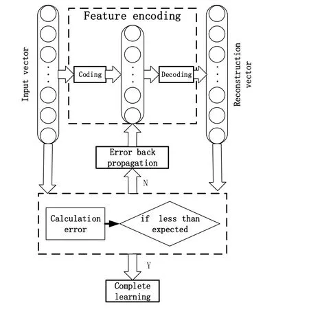
Figure 1: Auto-encoder

Where x and f(∙) denote the input sample and activation function, θ1={w1,b1}represents the network parameters, w1is the weight matrix and b1is the bias vectors.

Decoding is to propagate the feature encoding from the hidden layer to the output layer,then the k-dimensional vector ℎ will be mapped into m-dimensional vector by the activation function, finally, reconstruct the input sample and will obtain xˆ∈ [0,1]m×1,the decoding processing is as follows.

The goal of the AE network is to find a set of optimal parameters θ∗={w1∗,w2∗,b1∗,b2∗} which enable the output to be equal to the input data, that is to minimize the loss function(L(w1,w2,b1,b2)).

The first item in Eq. (4) represents the sum of the error with the input and output data of all training samples, where x(i)and xˆ(i)represent the input vectors and reconstruction vectors of the i-th samples. As shown in Eq. (5), J x(i),stands for the mean square error (MSE) between x(i)and xˆ(i). The second item in Eq. (4) is the regularization constraint item, it is used to prevent over fitting.

AE network minimizing the loss function L(w1,w2,b1,b2) by the error back propagation and the gradient descent method. The process of iterative optimization of AE network is as follows

Step 1: Initialize all the network parameters (w1,w2,b1,b2).

Step 2: Forward propagation and get the value of the hidden layer and the output layer neuron.

Step 3: Calculate the value of the error function L(w1,w2,b1,b2) in the current network state and determine whether the error is to achieve the desired minimum :If so, then the AE network is trained to complete and the current network parameters(w1,w2,b1,b2) are optimal; If it is not, do the next step.

Step 4: Calculate the residual error αi(3)of each neuron in the output layer of the network and the residual error αj(2)of each neuron node in the hidden layer, as shown in Eqs. (6)and (7). Based on the residual error, the residual error is propagated by the gradient descent method, and the network parameters w1,w2,b1,b2are updated, as shown in Eqs. (8) and(9).

Where in the Eqs. (6), (7), (8), (9),is the weight between the lth layer and the l+1t layer,stands for the bias between the lth layer and the l+1th layer and S3represents the number of neurons in the output layer; f(∙) is the activation function.

Step 5: Complete this iteration and return to Step 2.

2.2 De-noising auto-encoders

In reality, some part of the signal will lose the authenticity by the existence of noise (If the motor vibration signal is disturbed by the noise at a certain time, the feature of the signal will not express the motor state accurately.). Due to the above factor, the features obtained by AE method may be unreliable. De-noising Auto-encoder is to add noises to the training data on the basis of the Auto-encoder. The encoder needs to learn to get rid of noises so as to obtain the input signal which is not contaminated by noises, which makes it more robust.

First of all, according to the qDdistribution, the random noise will be added in the sample xn, such as Eq. (10).

Where, xis the corrupted input data. And x is achieved by means of a stochastic mapping of qD(x|x).

Then, the same as the traditional AE, it uses optimization algorithm to complete the network training by repeated iteration. In DAE method, we add random noise into the training samples. So, the influence of training samples and test samples distribution will be reduced, and the robustness of feature expression can be improved.

2.3 Stacked de-noising auto-encoder

Stacked De-noising Auto-encoder (SDAE) is stacked by many DAEs, the hidden layer of the above level DAE is used as the input layer of the next DAE, that is the feature vector of the above DAE hidden layer is used as the input of the hidden layer in next level, thus forming a multi-level network structure (Fig. 2). Bengio et al pointed out that different feature representation can highlight or remove some of the explanatory factors of the data,so that it can have different expression ability and multi-layer network structure can enhance the ability to distinguish the input data and weaken the non-related factors. So that to get the feature representation which is more suitable for task requirements.

The training of SDAE network: Firstly, input the initial data, train DAE1 network and get feature encoding h1; then, put the feature encoding h1 that get from the DAE1 network as the input of DAE2 network, and so on, put the feature encoding of DAE(n-1) network as the input of DAEn network, then training the DAEn network and get the final feature edcoding hn of the SDAE network.

The function of SDAE network is to feature encoding the input samples and strengthen the ability to distinguish the input data by the multi-times encoding of multi-layer network, which is conducive to better achieve sample classification. SDAE is an unsupervised network, which cannot complete the sample classification problem. In order to apply the SDAE network to the classification problem, the last layer of the SDAE network is coupled with a supervised network. As shown in Fig. 3, a supervised classifier(Softmax: will be introduced in the 2.3 Section) is added to the feature encoding of DAEn,so that the entire network becomes supervised.

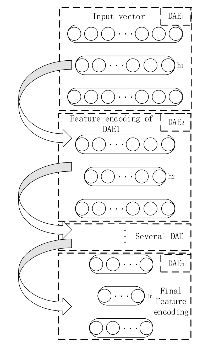
Figure 2: Network structure of SDAE

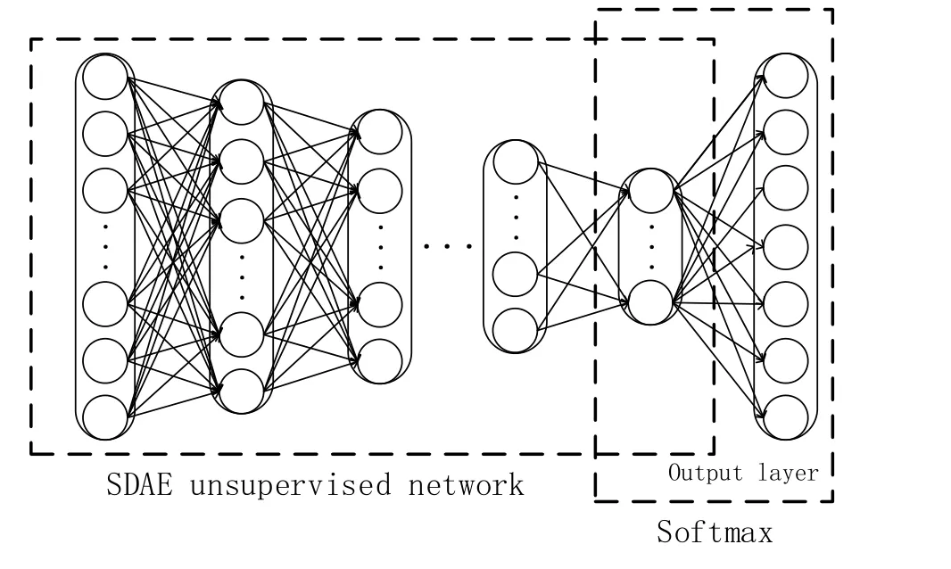
Figure 3: Supervised network

2.4 Classifier

Softmax is a generalization of Logistic classifier, mainly to solve the multi-classification problem. Suppose the input sample in the training data is x and the corresponding label is y. It will determine the sample j probability for a category for p(y=j|x). Thus, for a class K classifier, the output will be a vector of K dimension (The sum of elements in a vector is 1), as shown in Eq. (11).

Where,θ1;θ2;…;θk∈ ℜn+1are the parameter of our model; Notice that the termnormalizes the distribution, so that it sums to one.

In the training, after using the gradient descent method, the cost function of Softmax can be minimized by several iterations in order to complete the network training. The cost function J(θ) is shown in Eq. (12).

Where, 1{∙} is a indicative function, which means when the value of the braces is true, the result is 1; otherwise, the result is 0.

3 Model design and Signal preprocessing

The process of motor fault network training that based on SDAE is divided into 5 steps,with Fig. 4 showing the flow chart.

Step 1: Obtain the different fault signals of motor, then, take spectral analyzing, get the frequency domain signals as the input.

Step 2: Determine network parameters (such as network structure, learning rate, number of iterations, etc.).

Step 3: Layer by layer training according to motor fault features. In this paper, the number of hidden layer is N. The Auto-encoder neural network is trained sequentially.Let the output of DAE1 be the input of DAE2 and let the output of DAE2 (ℎ ℎ(x) )input to the classifier Softmax. According to the error of the network output and the expected target, the weight and bias term of each layer of the network are adjusted by the back propagation algorithm.

Step 4: Determine whether the accuracy meets requirements. If it meets, end the network training; if not satisfied, then adjust the network parameters and repeat the above steps(3).

Step 5: Complete network construction.

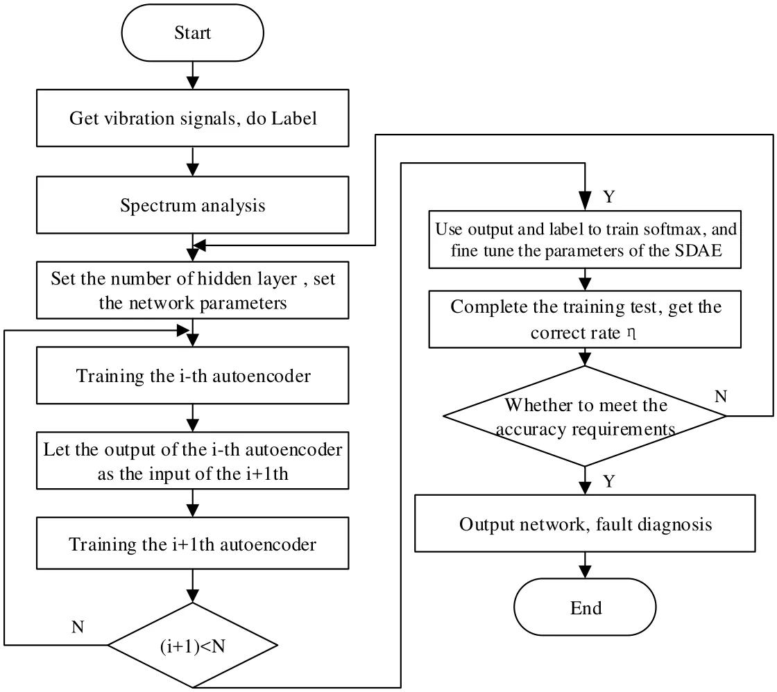
Figure 4: Flow chart of motor fault diagnosis

The input signals in this paper are frequency domain signals. Fast Fourier transform (FFT)is used to analyze the original signal in frequency domain to obtain frequency domain signals. The specific process is shown in Fig. 5.

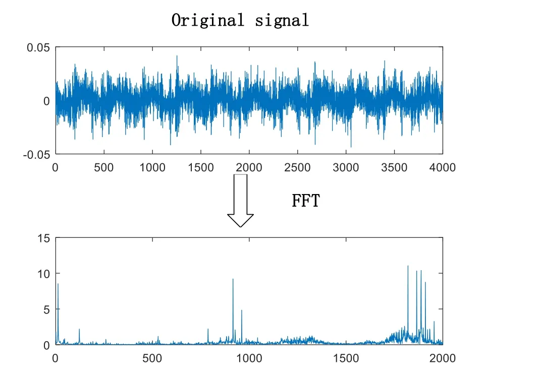
Figure 5: Signal preprocessing

4 Experiment and analysis

4.1 Data description

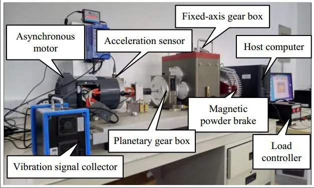
Figure 6: Drivetrain dynamics simulator system

In this paper, the research object is the Asynchronous motor in Drivetrain Dynamics Simulator system (Fig. 6) and the signal type is the vibration signal, we use SDAE method to monitor and diagnose their health status. The system consists of asynchronous motor, two levels of planetary gear box, fixed-axis gear box and magnetic powder brake.The sensor is installed on the right end of the motor. By changing the motor, we can simulate 7 different fault states. As shown in Tab. 1.For data acquisition, the working speed of the motor was 60 Hz, a sampling rate of 5 KHz was used for the motor faults. In order to ensure the diversity of the experimental data, 8 different working conditions were simulated when the data were collected correspond to 4 speeds (3560 RPM, 3580 RPM, 3600 RPM, 3620 RPM) and two different loads (have or not). Considering the influence of sensor position, two acceleration sensors are installed at the 9 o’clock and 12 o’clock positions on the right side of the motor (As show in Fig. 6).When selecting data, each working condition corresponds to 200 samples (each sensor contributes 100 signals). Thus, the total number of samples for each fault is 1600, the dataset contains 11200 samples. Each sample corresponds to the vibration signal of 4000 points.

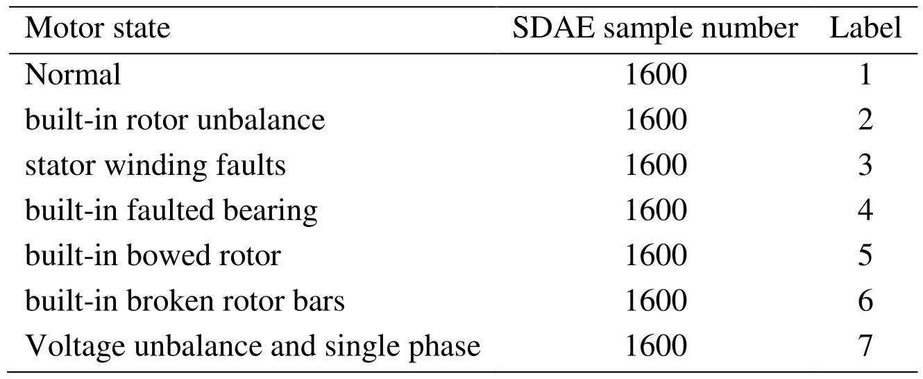
Table 1: Seven states of the motor

4.1.1 Fault description

We collected data on seven different health conditions of the motor (As shown in Tab. 1).These conditions involve normal, built-in rotor unbalance, stator winding faults, built-in faulted bearing, built-in bowed rotor, built-in broken rotor bars and voltage unbalance and single phasing. In each experiment, different motors were replaced, while the other components were normal.

Rotor unbalance is achieved by taking a balanced rotor from the manufacturer and intentionally removing balance weights and/or adding weight. The balance weights are attached to small aluminum pins protruding from both ends of the rotor. The bowed rotor motor consists of a motor with an intentionally bent rotor in the center 0.010. The faulted bearing motor consists of a motor with intentionally faulted bearings: One bearing with an inner race fault, and one bearing with an outer race fault. The broken rotor bar motor consists of a motor already fitted with an intentionally broken rotor bar. Enough material has been removed to expose three rotor bars. The motor has two windings with a 4V to 5V voltage difference which have been tapped to enable adding an additional load to the winding via an external control box. The control box consists of a 0-4 ohm variable resistor.The variable resistor or rheostat is used to introduce varying amounts of resistance in the turn-to-turn short between the windings, high resistance simulates an insulated winding and low resistance simulates a shorted winding. The phase loss and voltage imbalance is achieved by switching phases on and off; and introducing resistance with a control box.Simply connector the wire from the motor controller to the control box, and then connect the control box to the MFS. The phase loss switch opens the circuit to the first phase. The voltage control switch introduces a variable resistor of 0-25 ohm to the second phase. The third phase wiring remains untouched.

4.2 SDAE experiment and analysis

4.2.1 Number of hidden layers and nodes

In SDAE model, the number of hidden nodes and the depth of the deep architecture is normally of great importance to achieving high performance. Therefore, an experiment had been taken based on different hidden nodes and deep architecture. However, for better experimentation, all the other classifier model parameters are set as shown in Tab.2. Then, change the number of network layers and the number of nodes, and get the results shown in Tab. 3. It can be seen that when the first layer consisted of 1000 or 500,the error is too big, but when the nodes of first layer is 200 or 100, we can get better results.

The network structure should be as simple as possible, so focus on the first layer of the node to 100 of the situation. Through more experiments, we found that the effect of 3 hidden layers was significantly better than 2 and when the hidden layer is too much, the experimental effect may be reduced. Therefore, in order to ensure faster computing speed and less resource consumption, 3 hidden layer structures (100-100-50) are used.

Table 2: The SDAE classifier model parameters

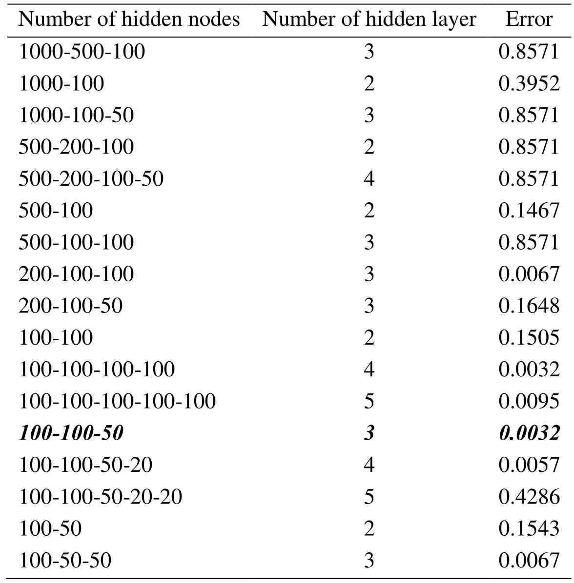
Table 3: Experimental result comparison with different hidden layer parameters

4.2.2 The selection of batch-size

Batch-size is an important parameter in deep learning. It represents the amount of data that is loaded at one time during training. The batch-size first determines the direction in which the gradient descends. When the data set is small, Full batch learning can be used.The direction determined by the full data set can better represent the sample population,so that it is more accurate to the direction of the extremum. However, for big data set,with the massive increase in data sets and memory constraints, it is becoming increasingly impossible to load all the data at once. So need to be trained in batches. But due to the sampling difference between the batches, the corrections for each gradient may cancel each other and cannot be corrected. In a certain range, in general, the greater the batch-size, the more accurate the descent direction, the smaller the training shock.However, blindly increasing the batch-size will reduce the number of iterations of an epoch, and the time it takes to achieve the same precision is greatly increased. Therefore,choosing a suitable batch-size not only improves accuracy, but also reduces the training time of the network. So we selected the batch-size as shown in Tab. 4 to experiment, In the best network structure (2000-100-100-50) and keep the other parameters unchanged.As can be seen from the table, when the batch-size reached 35, the accuracy rate reached the maximum and the time consumption is relatively small.

Table 4: Error under different batch-size

4.2.3 Noising mask probability

The method of adding noise in this method does not add the Gauss noise, Instead, the value of the input layer node is set to 0 with a certain probability. This method is similar to the commonly used Dropout in deep learning, but dropout works on the hidden layer.This way (SDAE) is similar to the human sensory system, such as when people look at objects, if a small part of the object is blocked, people can still identify it. This approach can improve the generalization ability of the network. The method of adding noise is used only in unsupervised training, not in fine tuning.

Figure 7: Error under different batch-size

In order to determine the best noising mask probability, we designed the following experiment (network structure: 2000-100-100-50, batch-size: 20, in addition to the noising mask probability, other parameters remain unchanged).

From Tab. 5, When the noising mask probability is very low, the error rate can be 0, but we suspect that the network may be overfitting. At this point, the generalization ability of the network is insufficient. To enable the network to have high generalization capability,we choose 0.6 as the appropriate probability of noising mask. (The choice of this parameter is conservative, and the research on the relationship between specific generalization ability and noising mask probability is not in this paper).

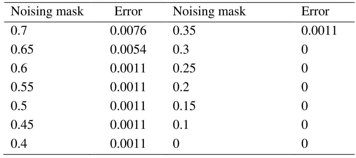
Table 5: Error under different noising mask

4.2.4 learning rate

In the process of training the SDAE, the gradient descent method is used for optimizing,learning rate is an important parameter that influences the adjustment of the weights and the convergence of the error. In order to improve the efficiency of network training, it is very important to select a suitable learning rate. However, as shown in Tab. 6, the learning rate is less affected under the current data set and parameters.

In the following experiment, we chose 0.5 as learning rate.

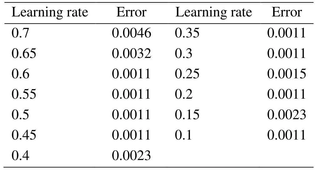
Table 6: Error under different learning rate

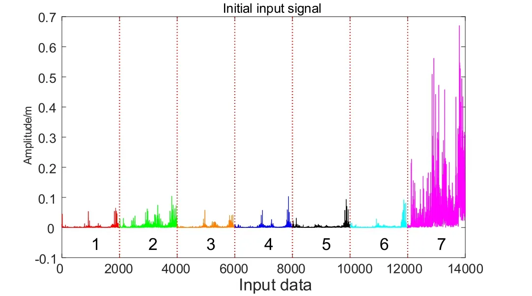
Figure 8: The frequency domain signal of each fault

4.2.5 Fine tuning

To further improve the classification performance, a back-propagation algorithm was used to fine tune the trained encoder. The network parameters are updated by minimizing training errors. The SDAE training process is divided into two steps: unsupervised training (Training the encoder layer by layer) and supervised training (Fine tuning). In order to explore the validity of fine tuning, we do feature visualization with the input samples of different faults by the trained network. So, we select one sample for each fault(as show in Fig. 8). Then, perform a forward operation, calculate the output of each encoder and print them.

Fig. 9 shows the seven different fault frequency domain signals, it is clear that the amplitude of the seventh failure is much larger than the first six. The second and seventh faults have more frequency domain components. The frequency domain signals of the 1,3, and 4 faults are similar, at the same time, 5 and 6 fault have a high degree of similarity.As show in Fig. 9, it is the output of three encoders with unsupervised training under 50 epochs (AE before fine tuning). and the output of the encoders after fine tuning. It can be clearly seen that the difference between the outputs of the various faults before fine tuning is not significant. But after fine tuning, there are very significant differences between the output of the various faults. It can be seen that the effect of fine tuning is obvious, it can improve the accuracy of the network.

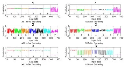
Figure 9: The output of each encoder before and after fine tuning

4.3 Research on feature visualization

In this particular section, we use the T-SNE method (Which is a kind of non-linear dimensionality reduction, which is to ensure that similar data points in high-dimensional space are as close as possible in low-dimensional space) to reduce each self-encoded output to 2-dimensional and print them out to represent different faults in different colors.The input of this experiment is for all test set data. As can be seen from the first figure of Fig. 10, after the first encoder, the fault data formed seven clusters. But it is clear that the blue and red clusters each have a gap. Then in the second figure, the clustering of each fault data is more closely (like a bar), but the red data showed a clear separation. Finally,after the third encoder, the apparent separation of red data is gone, all faults are well clustered into clusters. Thus, in dealing with high-dimensional data, SDAE has a good classification ability.

4.4 Comparative analysis between SDAE methods and other motor fault diagnosis methods

Feature extraction and pattern recognition are the two main processes of motor fault diagnosis. At present, the main methods of feature extraction are wavelet analysis,empirical mode decomposition and principal component analysis. We can also complete the feature extraction by analyzing the average motor signal variance, kurtosis, peak value and energy ratio. The methods commonly used in motor fault diagnosis are BP neural network and SVM.

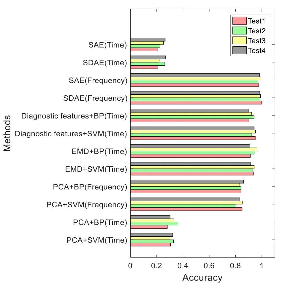
Figure 11: Cross validation results by each method

In order to compare with the traditional intelligent methods, in this paper, we also use EMD+SVM (BP) [Hu, Lou and Tang (2013)], PCA+SVM (BP), Diagnosis features+SVM (BP), and SAE for the motor fault diagnosis. Each method is compared with signal in time domain and frequency domain (The EMD method and the fault feature extraction method cannot be applied to frequency domain signals) The results are shown in Tab. 7 and Fig. 11.

PCA is a linear method in essence, and it is weak in dealing with the nonlinear problem.In this method, we select 8 feature components as the input of SVN and BP, and the PCA+SVM(BP) method has an unsatisfactory effect and its diagnostic accuracy is only 28%-36% for time-domain signal, and for frequency domain signals, the accuracy can reach 80%-86%. EMD can adaptive decompose signals, its essence is to obtain the eigen oscillation model through the characteristic time scale of signal, and then decompose the data. Therefore, it can only act in the time domain signal. And, either SVM or BP is used as classifier, the accuracy of the EMD method can reach more than 90%. For diagnostic features method, a strong prior knowledge is needed, and the original signals are statistically extracted to extract different features, the results under the two classifiers can both reach 90%-94%. As you can see from the Fig. 10 and Tab. 7, the SDAE and SAE methods have very poor effect when processing the time domain signals. From Tab. 5,we can see that when the noising mask is 0 (That is, the SAE method), the accuracy of the training set can reach 100%, but when the model is cross validated, the accuracy rate is not as high as that of the SDAE method. The accuracy of the SDAE method is nearly 1%higher than that of the SAE method. It shows that the robustness of the network can be enhanced by using the noise mechanism.

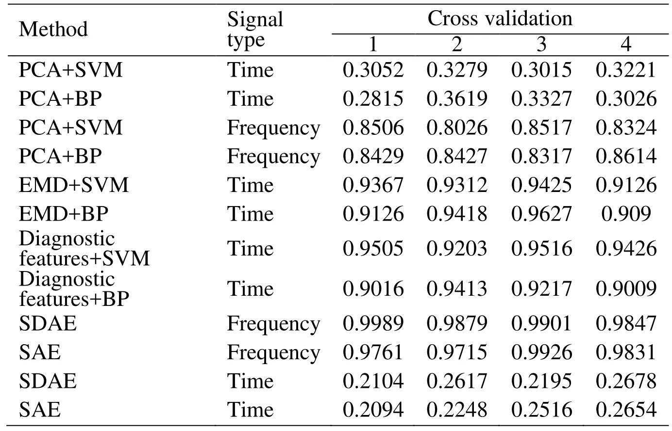
Table 7: Cross validation results by each method

5 Conclusion

In this paper, a deep learning method has been reported for motor fault diagnosis using Stacked De-noising Auto-encoder. Before the network training, we preprocessed the original signal and convert it into Frequency domain signal by Fourier Transform. By selecting different training parameters, an optimal one can be obtained to make the accuracy on the test set up to 99.89%, By comparing the diagnostic experiment results,the deep learning method used in this paper can adaptively extract the fault features and classify the faults with high accuracy. Through the study of feature visualization and compared with the traditional diagnostic methods. The advantage of the proposed approach is that by a universal learning process, rather than manually designed or with a priori knowledge of signal processing techniques, which is very useful for diagnosing problems.

Future work will include more experimental testing to further understand the limitations of the SDAE method. Especially in practical industrial applications, when faced with more complex faults. The choice of network structure and parameters is still an open problem.

Acknowledgment:This research is supported financially by Natural Science Foundation of China (Grant No. 51505234, 51405241, 51575283).