Subdivision of Uniform ωB-Spline Curves and Two Proofs of Its Ck−2-Continuity
2018-07-11JingTangMeiFangandGuozhaoWang
Jing Tang, Mei-e Fang, * and Guozhao Wang
1 Introduction
Polynomial B-splines and NURBS are important modeling tools in CAD/CAM. But polynomial B-splines are not able to exactly represent often-used conics (except for parabola), trigonometric functions and hyperbolic functions etc. NURBS can represent conics, but its ration form results in complicated computations about differential and integral. Then all kinds of B-like splines are proposed [Fang and Wang (2008); Zhang(1996); Vasov and Sattayatham (1999); Mainar and Pe˜na (2002)]. In paper [Wang, Chen and Zhou (2004)], we further unified these B-like splines into ωB-splines, which are constructed over. ω can be non-negative real number and pure imaginary number. If taking the value of ω as a constant 0,1 or i, we will get usual polynomial B-splines, trigonometric polynomial B-splines and hyperbolic polynomial B-splines respectively. ωB-splines inherit most of optimal properties from polynomial B-splines, including the subdivision property. Due to optimal properties of these B-like splines, many applications are studied in recent years [Mannia, Pelosi and Speleers (2012); Xu, Sun, Xu et al. (2017)]. In this paper, we perfect the subdivision method and theory of ωB-splines in order to apply them better in the future.
Subdivision is a standard technique of recursively generating smooth curves/surfaces from an initial polygon/mesh. Please see paper [Chaikin (1974); Doo and Sabin (1978);Catmull and Clark (1978); Dyn (1992); Stam (2001); Jena, Shunmugaraj and Das(2002);Jena, Shunmugaraj and Das (2003); Andersson, Lars-Erik, Stewart et al. (2010); Conti and Romani (2011); Conti, Cotronei and Sauer (2017)] for more details. This kind of modeling method is popularly applied in geometric modelling and 3D animation because of its numerical stability, simple implement and suitability for arbitrary topology. But most of subdivision curves and surfaces lack exactly mathematical representations, which are the fundamental of all kinds of differential/integral computations. So subdivision methods which have spline backgrounds are very interesting. Subdivision models with spline backgrounds include all merits mentioned above. For example, Doo-Sabin method[Doo and Sabin (1978)], Catmull-Clark method [Catmull and Clark (1978)], and the subdivision method proposed in paper [Stam (2001)] respectively have their spline backgrounds of B-splines of degree 2, cubic B-splines, polynomial B-splines of arbitrary order. These subdivision methods are all stationary, i.e, their subdivision rules persist unchanged in each level of subdivision. While stationary subdivision can not generate ωB-spline curves with frequency parameters.
In this paper, we introduce a parameter relative to the frequency parameter to build a nonstationary subdivision method with the background of ωB-splines. Then this kind of modeling method has the merits of both subdivision and ωB-splines. Concretely, we consider the subdivision of uniform ωB-splines with uniform knot intervals and ω taking a certain constant. At first, we derive the definition of uniform ωB-spline bases and curves according to the corresponding definitions in paper [Wang, Chen and Zhou (2004)].
Definition 1.1(uniform ωB-spline bases) LetTbe a given uniform knot sequencebe the length of uniform knot intervals,krefers to the order of splines .ωbe a given frequency parameter, where ω can take value as a non-negative real numberin this case) or a pure imaginary number whose imaginary part is positive.constructed by the following formula are called uniform ωB-spline bases in the span of.We first define uniform ωB-spline basic functions of orderk=2 as follows.
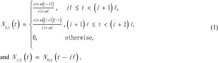
In formula (1.1), when ω = 0, we compute it by the L’Hospital rule about ω.
Definition 1.2(uniform ωB-spline curves) Letbe uniform ωB-spline bases of orderkcorresponding to the partitionthe parameter axis.
Thencalled an uniform ωB-spline curve of orderkcorresponding to the knot vectorT.are control points.ωB-spline curves can reproduce conics, trigonometric and hyperbolic curves. They also have many useful properties for geometry modelling, including those inherited from common B-spline curves and some special merits. Please refer to paper [Fang and Wang(2008)] for details. But we can see that the basic functions need to be recursively computed by integration from their definition, which results in low efficiency of evaluation. In this paper, we devote to build a high-efficiency subdivision method of generating ωB-spline curves.
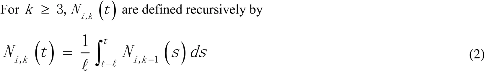
The rest of this paper is organized as follows. In Section 2, we derive the relation formula of control points between two representations of the same uniform ωB-spline curve of orderkrespectively with the original knot intervals and their bisections. Then the explicit subdivision rule is constructed based on this. By this kind of subdivision rule of orderk, a sequence of control polygons generates from the original control polygon of an uniform ωB-spline curve of orderk.We directly prove that the limit of this sequence converges to the-continuous uniform ωB-spline curve in Section 3. But this kind of proof method is hard to be applied in the corresponding proof of the continuity for the case of surface subdivision. So in Section 4, we reconsider the proof from the aspect of subdivision masks and provide a more general proof of the continuity of subdivision which will be easier to be extended to the case of surface subdivision. Because our proposed surface scheme is non-stationary, we use the theories of asymptotic equivalence between non-stationary subdivision and the corresponding stationary subdivision with the rule in limit status to complete the proof. The approximation order of the proposed subdivision scheme is also discussed. Section 5 makes a conclusion.
2 The subdivision method of uniform ωB-spline curves
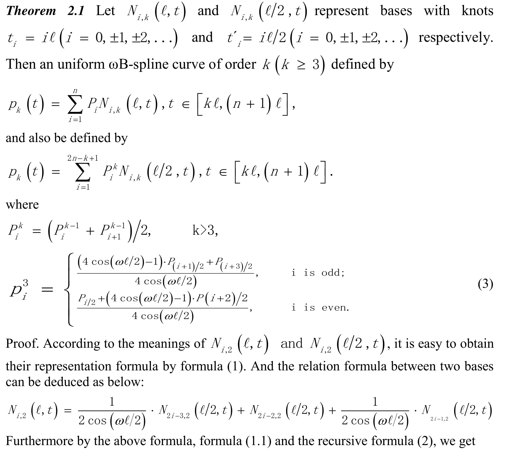
According to Definition 1.1 and Definition 1.2, we find that an uniform ωB-spline curve can also be equivalently represented by another uniform ωB-spline curve with knot intervals after bisection.

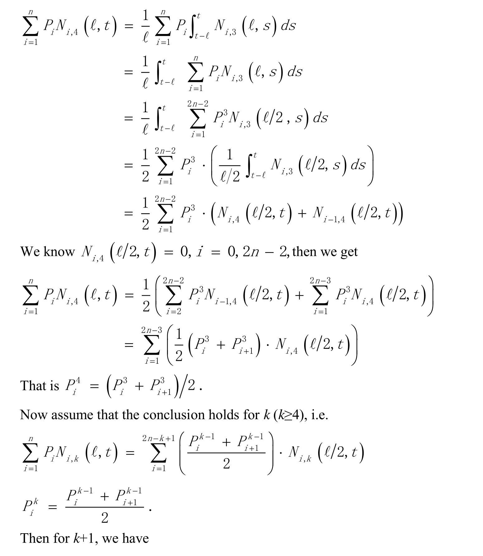
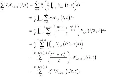
So the conclusion holds fork+ 1.
Based on this, an uniform ωB-spline curve can be generated by continuously using formula (4) from its initial control polygon. Letthe following definition of generating uniform ωB-spline curves by subdivision (ωBS for short).
Definition 2.1(ωBS scheme) Letbe the initial control polygon andbe the tension parameter. The subdivision rule of ωBS curves of order
is defined as:
式中:ak>0,取am=1.根据rkm的定义,当ak的赋值准确时,设评价指标xjk的权重系数wk,各指标的权重可以由以下公式确定:

Using the subdivision rule,the iterative process of ωBS is described as below.
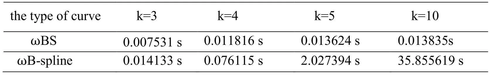
Table 1: The time report of generating ωBS curves and ωB-spline curves from the same control polygon
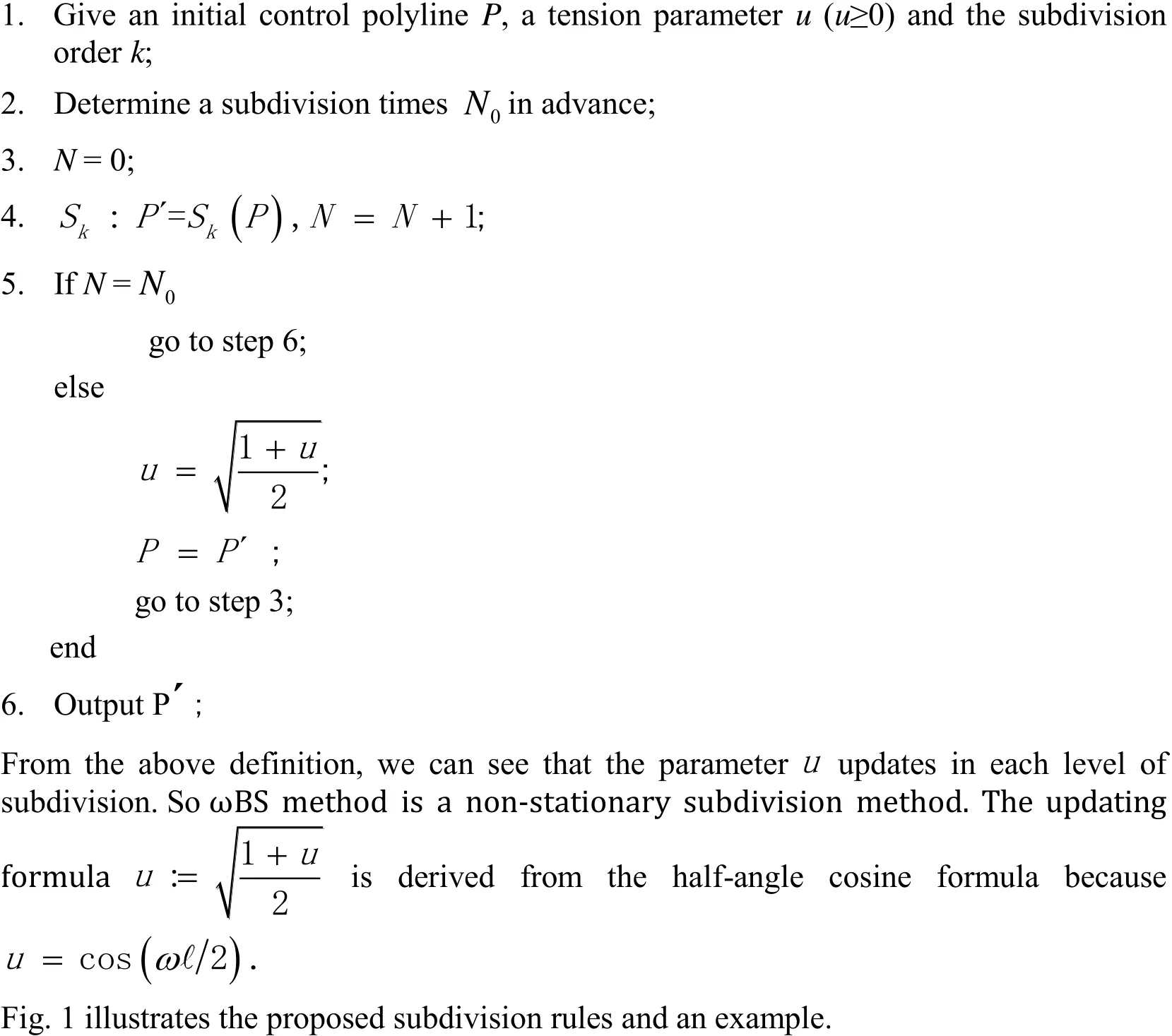

Figure 1: The subdivision rules (a)(b)(c) and an example (d)(e)(f).
In Fig. 1 (a),is computed by formula (5) from the initial control polylineis computed by formula (5) fromSimilarlycan be computed by formula (5) fromIn Fig. 1(c),the black poly lines are respectively the results after one level and two levels of subdivision from the initial control poly line whenk=5,u=3. The red curve is the results after six levels of subdivision which can be seen as the approximation of the limit curve.The green and purple curves respectively correspond to the cases ofk=5,u=1 andk=5,u=0.5. In Fig. 1(d), the profile of an industrial model which consists of three pieces of circular arcs (red), some line segments and some cushioning curves. In Fig. 1(e), the control polygon of the profile is computed according to the ωB-spline representation proposed in paper [Fang and Wang (2008)]. In Fig. 1(f), the profile is reproduced by subdividing the control polygon according to the proposed method in this paper,
Comparing Definition 2.2 with Definition 1.1 and 1.2, we can see that ωBS curves only include linear computations, which is much simpler and more efficient than those recursive integral computations included in the definition of uniform ωB-spline bases.This is very important for real-time rendering and hierarchically displaying curves and surfaces. Taking the control polygon illustrated in Fig. 1(e) with 33 control points as an example, Tab. 1 shows the comparison of the efficiency of both methods to render the curve jointed with the same number (about 300) of points. Apparently, the efficiency of rendering ωBS curves is much faster than rendering ωB-spline curves. And with the increase of order, the difference between them becomes bigger and bigger.
From Theorem 2.1, we know ωBS curve is derived by the knot interpolation method of uniform ωB-spline curves. The sequence of control polygons formed by continuous bisections of knot intervals will converge to smooth ωB-spline curves, which are-continuous. That is to say, ωB-spline curve is the limit curve of ωBS curve with the same control polygon when the subdivision level tends to infinity. In the next two sections, we prove that ωBS curves are alsocontinuous using two proving methods.
3 One proof of C k−2 -continuity of ωBS curves
Theorem 2.1 shows how the new control polygon can be obtained from the old control polygon after a round of subdivision. We have the following theorem.


Proof. Based on Definition 2.1 and Theorem 3.1, we can conclude that ωBS curves of orderk(k≥3) converge to uniform ωB-spline curves of order k whose-continuity are obvious according to the definition of ωB-spline basis functions and paper [Wang,Chen and Zhou (2004)]. So the conclusion holds.
4 Another proof of -continuity of ωBS curves
The proof in Section 3 is simple. But this proof method is difficult to be extended to the case of surface subdivision, especially non-tensor product surface subdivision. So we provide another proof method for-continuity of ωBS curves based on those theories upon subdivision masks, which will be advantageous to be applied in the proof of our further surface subdivision.
From the steps of ωBS described in Definition 2.2, we can see that the tension parameter is changing with the subdivision level, so ωBS is a non-stationary subdivision scheme.For convenience of proving its continuity, we introduce the corresponding notions of the mask of ωBS at first.


It can be easily checked that the support of the maskis indeed the same as the one of the classical B-spline of orderk[Stam (2001)].
It’s difficult to directly prove the continuity of a kind of non-stationary subdivision scheme. So we prove-continuity of ωBS curves according to the theorems including asymptotic equivalence proposed in paper [Dyn and Levin (1995)]. Here we cite the notion of asymptotic equivalence between two schemes defined in paper [Dyn and Levin (1995)].


This is the mask of the Chaikin’s corner cutting algorithm and it generateslimit curve(see Chaikin [Chaikin (1974); Dyn and Levin (1995)]). Now, to estimate the-smoothness of the proposed scheme of order 3, it is necessary to estimate the difference betweenand. From (9), we see that
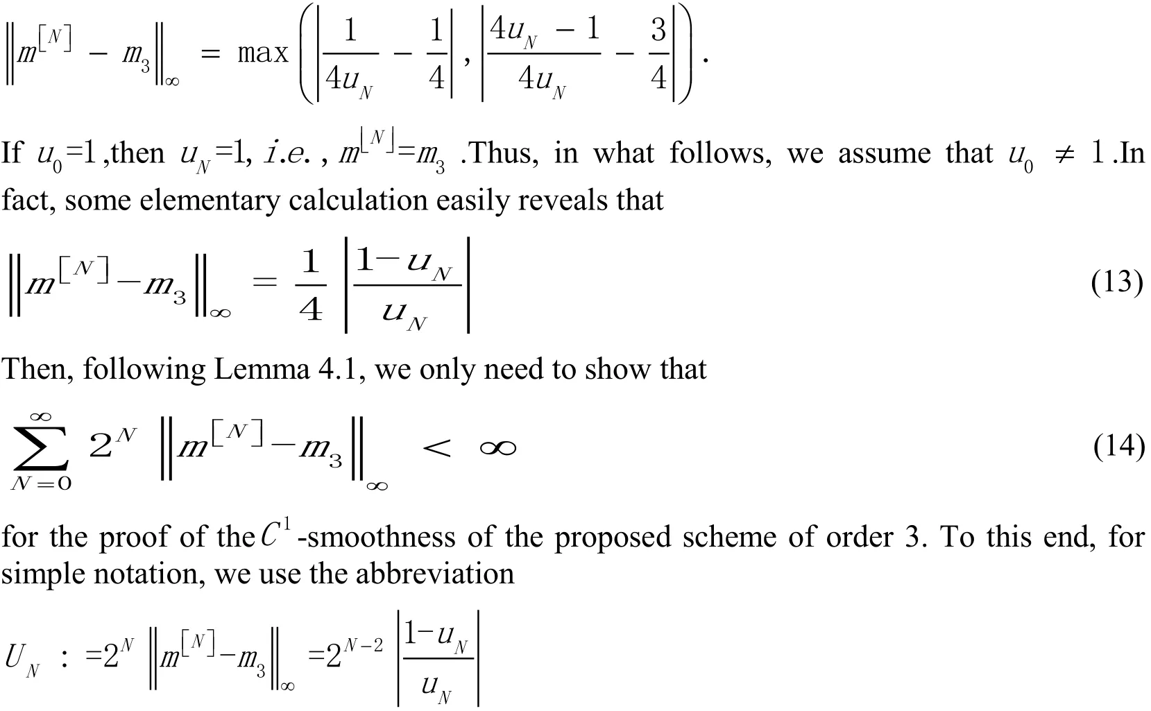

Following the D’Alembert criteria for convergence of positive series and in view of (13),the claim (14) is proved.
We are now ready to prove the smoothness of the proposed scheme of orderk>3. In the following analysis, we will see that it is convenient to represent a subdivision rule with the maskin terms of the symbol
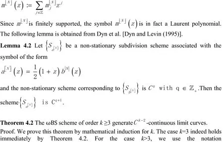

wherehe symbol of the ωBS scheme of order 3 with the mask(10).By Theorem 4.1, the scheme associated to the Laurent polynomialHence, applying Lemma 4.2 inductively, we can conclude that the proposed scheme of order k is.
The approximation order of the proposed non-stationary subdivision is also important. In the following, we discuss this problem. Theorem 4.3 shows that it is of approximation orderk-1, wherekrefers to the order of the corresponding ωB-splines.
Theorem 4.3 For the ωBS schemef orderk≥ 3, the approximation order of this non-stationary subdivision isk-1.
Proof.Based on Lemma 4.1, the proposed non-stationary subdivision scheme is asymptotically equivalent to a stationary schemeconverges to ωB-splines of orderk, with a constant frequency sequence, which can reproduce polynomials of orderk-1.According to the results concluded in paper [Conti, Dyn, Manni et al. (2015); Conti,Romani and Yoon (2016)], we know a non-stationary subdivision implies approximation order k-1 (k-1 refers to the degree of ωB-splines) asymptotic similarity to stationary scheme is assumed. So based on the above, the conclusion of Theorem 4.3 is proved.
5 Conclusion
In this paper, we proposed the subdivision scheme for uniform ωB-spline curves. Then a uniform ωB-spline curve has both perfect mathematical representation and efficient generation method. We also provide two proofs of-continuity ωBS curves ofkorder in two different aspects and discuss its approximation order. The first method is direct and simple. The second kind of proof is based on subdivision masks and some corresponding theories, which will be advantageous to prove the corresponding conclusions of surface subdivision. In the future, we will extend the subdivision scheme to the case of surfaces with tensor product form and further arbitrary topology as well. In addition, we will apply ωB-splines and especially the subdivision scheme in the all kinds of applications relative to finite element method (FEM) and isogeometric analysis (IGA)to improve the accuracy during modeling and analysis [Wang, Shen, Zou et al. (2018);
Guo and Nairn (2017); Xu, Sun, Xu et al. (2017)].
Acknowledgement:The work described in this article is partially supported by the National Natural Science Foundation of China (61772164, 61761136010) and the Natural Science Foundation of Zhejiang Province (LY17F020025).
Andersson, L. E.; Stewart, N. F.(2010): Introduction to the mathematics of subdivision surfaces.Society for Industrial and Applied Mathematics, Philadelphia.
Catmull, E.; Clark, J.(1978): Recursively generated B-spline surfaces on arbitrary topological meshes.Computer Aided Design, vol. 10, no. 6, pp. 350-355.
Chaikin, G. M.(1974): An algorithm for high speed curve generation.Computer Graphics and Image Processing, vol. 3, no. 4, pp. 346-349.
Conti, C.; Dyn, N.; Manni, C.; Mazure, M. L.(2015): Convergence of univariate nonstationary subdivision schemes via asymptotic similarity.Computer Aided Geometric Design,vol. 37, no. 6, pp. 1-8.
Conti, C.; Romani, L.(2011): Algebraic conditions on non-stationary subdivision symbols for exponential polynomial reproduction.Journal of Computational and Applied Mathematics,vol. 236, no. 4, pp. 543-556.
Conti, C.; Romani, L.; Yoon, J.(2016): Approximation order and approximate sum rules in subdivision.Journal of Approximation Theory, vol. 207, no. 2, pp. 380-401.
Conti, C.; Cotronei, M.; Sauer, T.(2017): Convergence of level-dependent hermite subdivision schemes.Applied Numerical Mathematics, vol. 116, no. 1, pp. 119-128.
Doo, D.; Sabin, M.(1978): Behaviour of recursive subdivision surfaces near extraordinary points.Computer Aided Design, vol. 10, no. 6, pp. 356-360.
Dyn, N.(1992): Subdivision schemes in computer-aided geometric design. In:Advances in numerical analysis: Volume II: Wavelets, subdivision algorithms and radial basis functions.Clarendon Press, Oxford.
Dyn, N.; Levin, D.(1995): Analysis of asymptotically equivalent binary subdivision schemes.Journal of Mathematicl Analysis and Application, vol. 193, no. 2, pp. 594-621.
Fang, M.; Wang, G.(2008):ωB-splines.Science in China Series F: Information Sciences, vol. 51, no. 8, pp. 985-1102.
Guo, Y.; Nairn, J.(2017): RETRACTED: Simulation of Dynamic 3D crack propagation within the material point method.Computer Modeling in Engineering & Sciences,vol.113, no. 4, pp. 389-410.
Jena, M. K.; Shunmugaraj, P.; Das, P. C.(2003): A non-stationary subdivision scheme for generalizing trigonometric spline surfaces to arbitrary meshes.Computer Aided Geometric Design, vol. 20, no. 2, pp. 61-77.
Jena, M. K.; Shunmugaraj, P.; Das, P. C.(2002): A subdivision algorithm for trigonometric spline curves.Computer Aided Geometric Design, vol. 19, no. 1, pp. 71-88.
Mainar, E.; Pe˜na, J. M.(2002): A basis of C-Bezier splines with optimal properties.Computer Aided Geometric Design, vol. 19, no. 4, pp. 161-175.
Manni, C.; Pelosi, F.; Speleers, H.(2012): Local hierarchical h-refinements in IgA based on generalized B-Splines.International Conference on Mathematical Methods for Curves & Surfaces, vol. 8177, no. 4, pp. 341-363.
Stam, J.(2001): On subdivision schemes generalizing uniform B-spline surfaces of arbitrary degree.Computer Aided Geometric Design, vol. 18, no. 5, pp. 383-396.
Vasov, B. K.; Sattayatham, P.(1996): GB-splines of arbitrary order.Journal of Computational and Applied Mathematics, vol. 1, no. 1, pp. 155-173.
Wang, C.; Shen, Q.; Zou, Y.; Li, T.; Feng X.(2018): Stiffness degradation characteristics cestructive testing and finite-element analysis of prestressed concrete T-beam.Computer Modeling in Engineering & Sciences, vol. 114, no. 1, pp. 75-93.
Wang, G.; Chen, Q.; Zhou, M.(2004): NUAT B-spline curves.Computer Aided Geometric Design, vol. 21, no. 2, pp. 193-205.
Xu, G.; Sun, N.; Xu, J.; Hui, K.; Wang, G.(2017): A unified approach to construct generalized B-Splines for isogeometric applications.Journal of Systems Science &Complexity, vol. 30, no. 4, pp. 983-998.
Zhang, J.(1996): C-curves: an extension of cubic curves.Computer Aided Geometric Design, vol. 13, no. 3, pp. 199-217.
猜你喜欢
杂志排行
Computer Modeling In Engineering&Sciences的其它文章
- Progressive Failure Evaluation of Composite Skin-Stiffener Joints Using Node to Surface Interactions and CZM
- The Reduced Space Method for Calculating the Periodic Solution of Nonlinear Systems
- Online Group Recommendation with Local Optimization
- Exact Solutions of the Cubic Duffing Equation by Leaf Functions under Free Vibration
- A New Interface Identification Technique Based on Absolute Density Gradient for Violent Flows