An efficient aerodynamic shape optimization of blended wing body UAV using multi- fidelity models

Parviz MOHAMMAD ZADEH,Mohsen SAYADI

Faculty of New Sciences and Technologies,University of Tehran,Tehran 1439957131,Iran

1.Introduction

In recent years,in order to reduce fuel consumption and improve the performance,the optimization of UAV shapes has been the main focus of the competitive aerospace market.The development of Blended Wing Body(BWB)design is such an effort.In addition to the elimination of the tail for this particular kind of UAV and the significant reduction in equivalent weight,drag force,and radar cross-section,the available space for installing equipment inside the wing and the effective rangehave also been increased.Despite all these mentioned advantages,instability is the negative outcome of eliminating the tail.Correcting this flaw requires designing a combination of control surfaces and reflexed wing sections and using sophisticated computer control systems.Therefore,the aerodynamic shape design optimization of BWBs,along with the need to meet the design requirements,has inspired several researchers to overcome its challenges.

However,BWB and pureflying wing have some differences in definition;their optimization design approaches and some principles of aerodynamic design are practical for each other.The BWB design challenges along with necessity of developing aircraft efficiency impose more computational effort on the preliminary design process.

Various objectives and different constraints in the design of BWB make them a proper candidate for the application of multi-objective and multi-disciplinary design optimization techniques.1,2The characteristics of their shape makes their geometry parameterization easier.A study on improving the Concurrent Subspace Optimization(CSSO)structure on the basis of response surface and Monte Carlo analysis for the robust,single-objective optimization of the flying wing was conducted in this field.3Multidisciplinary Design Optimization(MDO)architecture of aerodynamic shape optimization was developed for battery-powered composite BWB with Delta wing.4The results of implementing this architecture and conventional optimization process were compared to demonstrate the presented formulation.Pan et al.5presented a systematic technique in aerodynamic and stealthy MDO issue for double-sweep flying wing.They utilized the hybrid structure of global optimization and gradient algorithm as an optimization strategy in conceptual design.Morris et al.6devoted attention to multi-disciplinary multi-level optimization for the simultaneous optimization of aerodynamic shape and structure.

The mere design of the aerodynamic shape was the main objective of optimization in certain studies,while only the airfoil cross-section was the focus in some others.7,8The definition of geometry and surface meshing was investigated by Truong et al.9to enhance the quality of the mesh modified during optimization.The robust design of airfoil shape optimization is investigated to reduce the sensitivity of small random geometry perturbations and uncertain operational conditions.10The construction of meta-models based on Kriging and gradient-enhanced Kriging is based on a relatively small number of CFD evaluations.Since the optimization of the fixed geometry aircraft demands satisfying conflicted constraints in various flight conditions,aerodynamic shape optimization of morphing wing is the subject of the study by Hunsaker et al.11This method increases allowable wingspan with induced drag reduction for a given structural weight.

In addition to putting forward an optimal Lifting-Fuselage Con figuration(LFC)shape for BWB in the research by Reist and Zingg,12the aerodynamic shape was optimized for the best cruise altitude and reduced fuel consumption.In another study,the hybrid design of the aerodynamic shape and structure of the flying wing was optimized by combining the multi-bump method with automatic optimization and flow control to increase the lift-to-drag ratio and improve longitudinal static stability.13The presented approaches differ mainly in the definition of the geometry of the problem,objective functions,optimization constraints,14and finally,the accuracy of the adopted models.15

In complicated engineering design problems such as BWB,Surrogate-Assisted Optimization(SAO)methods have been developed to enhance the accuracy and reliability of optimization process.16In particular,due to the high computational cost of solving the CFD models,the researchers use the meta-model in aerodynamic optimizations.14,17,18However,constructing accurate meta-modelwould stillbe timeconsuming and is often associated with insufficient accuracy in order to ensure a great degree of change in variables and the presence of local extrema for the objective and constraint functions.

The concept of sequential approximation method is introduced to overcome the mentioned limitations of the metamodels imposed by large-scale and complex design space.19The simulation outcomes show that building appropriate low- fidelity model reduces the computation costs and improves model accuracy.Using the response correction techniques for aerodynamic shape optimization introduced by Koziela et al.7,the precision of the alternative models derived from lowaccuracy models is improved.An automated selection of low- fidelity model for aerodynamic shape optimization is proposed in another study.20This approach utilizes low-and highfidelity model misalignment.

In the variable- fidelity shape optimization,the hierarchical kriging technique is utilized for modifying low- fidelity kriging model.21Since the low- fidelity model is constructed based on a single design point,some weighted aerodynamic data correct the meta-model as high- fidelity data.Other studies consider the effects of boundary layer transition for optimizing the shape of a lifting body with adjustment of the metamodels.22The sample selection method for correcting the model plays a key role in such architectures.23Maximizing the Expected Improvement function(EI),24Probability of Improvement function(PI),and the Mean Squared Error(MSE)25and minimizing the Lower Confidence Bound(LCB)26are some examples of these methods—known as in filling strategies.

K-means algorithm classifies the solutions for selecting points and modifying the database of the meta-model,whereas genetic algorithm is tasked with optimization of the aerodynamic shape.27The application of the parallel processing capabilities to the optimization of aerodynamic problems is facilitated by combining these techniques in order to mitigate the defects of each.23,28

The other method for reclaiming local adaptive meta-model building is the move-limit strategy.The main merit key of these approaches is the suppression off design space in the current optimum point neighborhood and re fining of the model in this space.The vital importance of selecting the move limit strategy is controlling optimization performance.These strategies—both fixed29and adaptive30—differ from one another by different bound-adjustment methods.31Among them,the global convergence can be achieved by utilizing the trust-region method.32

On the other hand,the selection of design variables in shape optimization has an important effect on the appropriate covering design space and reduction of computational cost.Poole et al.33proposed a novel method for the proper orthogonal decomposing set of training airfoils,which increase the number of the required shape optimization variables based on an optimal set of airfoil deformation modes.

Although gradient-based algorithms are very popular due to their higher computational speed in solving aerodynamic problems,evolutionary algorithms,such as genetic algorithm34and particle swarm optimization,35have been employed in a number of studies.It should be taken into consideration that the use of these algorithms would be more cost-effective owing to the great number of evaluations in multi-objective problems,while they offer a better guarantee of evading the local minima.36On the other hand,numerous studies have been conducted to decrease the computation time of gradientbased algorithms.The presentation of the adjoining method was such an effort37that was associated with the calculation of the derivative of aerodynamic forces.The Sparse Nonlinear OPTimizer(SNOPT)algorithm—a combination of this method with SQP method—has received much attention from researchers.38,14

To enhance the aerodynamic shape design optimization of BWB UAV,an adaptive robust design optimization framework is presented in this paper.In the proposed framework,initializing global meta-models from the 2D low- fidelity model significantly reduces computational costs,while locally tuning meta-models with high- fidelity models increases model accuracy near the global optimum point.Since the proposed framework employs 3D high- fidelity models to construct local metamodels,a promising reliability can be accomplished.In addition,in each optimization iteration,the adaptive trust region manages space design and the uniformed sampling technique guarantees the model’s robustness.

2.Methodology

The main aim of this paper is to reduce computational time for solving aerodynamic shape optimization based on 3D high fidelity aerodynamic model.Towards this goal,the approach adopted in this paper involves first utilization of sensitivity analysis to eliminate the design variables,which have very low impact on the objective function(i.e.,CD)or the constraints.Therefore,the design variables,which were eliminated from the optimization process have very low impact effect on the objective function(i.e.,CD)and constraints and this is mainly used to reduce the computational time.Second,this paper presents accurate meta-models using multi- fidelity modelling to reduce the computational time significantly and at the same time to achieve accurate CDbased on high fidelity(3D)aerodynamic model.The approach is adopted based on two levels of meta-model building process(i.e.global and local).One of the key advantages of the multi- fidelity modelling approach presented in this paper is the use of models of different fidelity,i.e.low- fidelity(panel model)and high- fidelity(3D)aerodynamic models in the optimization process.In the proposed method,the interaction between 2D and 3D aerodynamic models is utilized to correct(tune)2D aerodynamic model to achieve the same degree of accuracy of the 3D aerodynamic model,but at the same time it is computationally very efficient model to be used in the aerodynamic shape optimization process.

Fig.1 illustrates the framework of the proposed optimization technique for the aerodynamic shape optimization of BWB UAVs.This framework is not limited to aerodynamic optimization and can be implemented for other types of geometric optimization.According to this,optimization process is partitioned into three stages.In the first stage,the initial design geometry is parameterized and high- fidelity and lowfidelity models are derived.The aim of the second stage is to construct the global meta-model from the low- fidelity model.Finally,the local meta-model is tuned in the neighborhood of the current design point to improve the accuracy in each optimization iteration.

Regardless of the optimization nature,each optimization problem begins with the mathematical definition of the problem’s objectives and constraints.How the problem is defined,i.e.optimization problem definition,affects the solution process and the final optimal solution.Generally,an optimization problem aims to minimize an objective function f（x）and satisfy the constraints of equality(h（x）)and inequality(g（x）).According to the problems,the functions may be linear and/or nonlinear,as defined in the following:

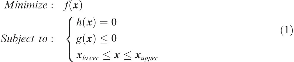
where x is the vector of design variables with the length of n,and xlowerand xupperare the upper and lower limits of the variables,respectively.

The implementation method of the structure introduced for the problem is elaborated in the subsequent sections.

2.1.Preparing geometric models

The first step in this study is the appropriate definition of 2D(low- fidelity)and 3D(high- fidelity)geometries.The defined models should have all the specifications as well as an automatic geometric parameterization.In fact,all the geometric variables(geometric dimensions)should be defined parametrically,so that the overall geometry changes automatically and in proportion to other variables,as the value of each variable changes.

This study considers appropriate control points at the selected sections.Regardless of the number of changes in the position of control points,the final shape is a smooth surface passing through the control points.On the other hand,by defining appropriate constraints along the third dimension,taper ratio and the distances of control sections change not only individually,but also across the whole shape with respect to the final geometric shape.Therefore,the final shape undergoes distortions both in the 2D sections and in the 3D space related to variable change.

However,improving the accuracy of a model involves an exponential increase in the computational cost.Therefore,the defined model should be simple and a reflection of the actual behavior.The main idea of the introduced framework is the application of a low- fidelity model(2D model),which leads to a simpler closed form.

The low- fidelity 2D model is extracted by simplifying the high- fidelity 3D model.In fact,in this model,similar sections of the 3D model are selected to define shape points,while design variables are defined corresponding to them.Since the panel method evaluates each section and the results are ultimately collected to obtain the values of objective functions and constraints,the amount of calculations required is decreased.By comparing results of 3D and 2D models,the correction factor(model’s modifier coefficient)is derived.This modification improves the accuracy.

Fig.1 Efficient aerodynamic shape optimization of BWB UAV using multi- fidelity models.

2.2.Initializing global meta-model

The optimization of aerodynamic shape still takes a long time,even when low- fidelity models are utilized.Employing the meta-model is one of the situated strategies to diminish computational time in the optimization process.On the other hand,in large-scale and complex problems such as aerodynamic optimization,the number of design variables is another factor that affects the convergence specification and gradually increases computationaltime.Consequently,the nonprominent variables can be eliminated by means of ANOVA for simplification of the meta-model.In this technique,it is assumed that the explicit function f can be decomposed as expressed in the following form:

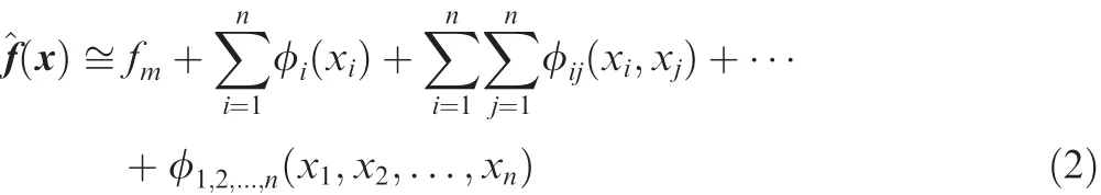
where fmand φ are the means of output distribution and lowdimensional decomposition terms respectively.The contribution indices πkbased on smoothing spline ANOVA are interpreted as importance of decomposition terms and are defined below:

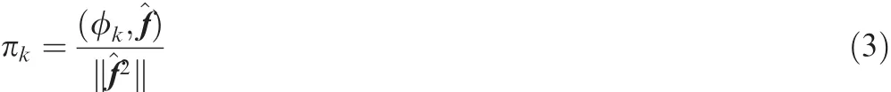
where （·，·）and||.||are the scalar product of vectors and vector norm respectively.The effective terms have a higher value that would be kept,while the lower value shows a negligible effect that should be eliminated.39

The sampling points would be as well-distributed as possible in design space.Full or fractional factorial design,central composite design,Taguchi,40Sobol41and uniform Latin Hypercube42are some of the predominant Design of Experiments(DoE)schemes.The uniform Latin hypercube method has been suggested for ensuring the evenness of the sampling points.This DoE approach explores the entire design space without taking into consideration the dimension of the problem.

The meta-model features can be significantly affected by the selected construction method.Polynomial regression,43moving least-square method,44neural networks,fuzzy logic,45kriging,46and radial basis function47are some of these approaches.48Kriging method is utilized by several aerospace researchers to build a high-quality meta-model.49In this study,based on the Gaussian process theory,this method is preferred compared with the other ones.At higher dimensionality like wing design,this method has promising performance and more robustness in constructing meta-models and updating them as well as in lowering the computational time.50

The key factor in accuracy and convergence rate of optimization methods such as Sequential Quadratic Programming(SQP)is the selection of initial point.Selection of a feasible point as the starting point may also prevent confusion of the optimizing algorithm and reduce the computational costs.Therefore,DoE sample with the smallest value of the objective function is selected as the initial point.

2.3.Optimization process

Iterative optimization by updating a meta-model is taken into consideration to achieve a structure with optimal performance.In any iteration of optimization process,SQP optimization algorithm determines the optimal point in proportion to the problem conditions.On the other hand,meta-model parameters are modified locally in the neighborhood of the optimal point found in the design space.In other words,the modified model is optimized in the created trust region of the local meta model in the following stage by assuming the current optimization point as the initial point.In other words,the optimization process continues as long as the local meta-model and the optimal value are fixed.

2.3.1.Global optimization algorithm(AFSQP)

Adaptive Filter Sequential Quadratic Programing(AFSQP)is an algorithm based on SQP with adaptive filter,which is extensively used for the global optimization of single-objective nonlinear constraint problems.The advantage of this method overshadows the performance of nearly all other nonlinear programming methods in terms of velocity,accuracy,and percentage of feasible solutions.51Taking the optimization history into account and inspired by the idea of multi-objective optimization problems and the adaptive adjustment of the number of inputs to the filter during optimization,AFSQP provides the only dominant point compared to previous solutions.52Hence,x＊is the optimal point of the problem if it satisfies:

where λ*is the optimum value of Lagrange multiplier.

The main steps involved in optimization with AFSQP are described below:

Step 1.Determine the initial point.Design variable bounds,the maximum number of iteration,and termination tolerance on the function value and constraints violation.De fine the scalar-valued ‘Lagrange function” in the following form:

Step 2.Formulate QP problem for the iteration （k）and the unknown linear search direction d

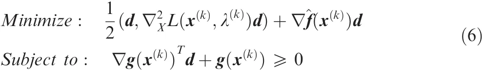
Step 3.Solve QP problem Eq.(6),d value.The tentative point is x（k+1）=x（k）+d.

Step 4.If tentative point does not pass the test,appropriate reduction is applied and α value controlled.The adaptive filter judges the next iteration safety, αnew=rαold.The optimal choice of reduction factor,r∈(0,1),is discussed by Truco.53An evolutionary scheme adapts parameter r in a randomly adaptive perturbation manner.The promising solution is expressed as

Step 5.The constraint violations are reduced with feasibility restoration.By introducing slack variable,the solution of iterative trust-region algorithm is transformed.54This step is invoked when the filter accepts point or the constraint violations satisfy threshold criterion.

Step 6.Until any termination condition,such as achieving termination tolerance on the function value or maximum number of iteration,is met,the number of iterations is incremented by+1 and then Step 2 is repeated.

2.3.2.Tuning local meta-model

Improving the accuracy of calculations leads to an improvement in the accuracy of the model.In this way,the metamodel is updated after each optimization stage.In the proposed method,updating is based on a few solutions of the high- fidelity model to affect the model accuracy in a better way.In fact,by limiting the variable bounds and modifying the database,parameters of the meta-model are adjusted locally,neighboring the optimal point.Therefore,the modified meta-model ofis a function of the evaluations of the highifdelity model of f(x)and the existing meta-model of）in the new design.

Selection of points to modify the high- fidelity model database was done based on move-limit strategy method,described in detail below.

2.3.3.Move-limit strategy

Sequential approximation method is one of the most practical methods used to improve the accuracy of meta-model for increasing the convergence probability under reduction of the computational time caused by iterative analysis costs.It is sometimes very difficult to find a meta-model with sufficient accuracy throughout the design space.55The theory of this method is based on suppressing variable boundaries in the neighborhood of the current design point.The modified boundary,called ‘trust region”,is determined in each stage based on solution positions.Therefore,optimization is performed locally and there are limited permissible changes in design variables.In other words,they are move-limited.Selection of move-limit strategy,especially when model accuracy is insufficient,plays a crucial role in controlling convergence rate.34

In this method,the current optimal point is at the center of the new design space and new sampling points are distributed in this space.A new algorithm called ‘Adaptive Uniform In filling”is presented for the proper distribution of the points in the new space.

The number of the points selected during optimization is adaptively determined in relation to the number of optimization iterations.Therefore,the number of required sampling points reduces adaptively by limiting variable boundaries corresponding to model accuracy and eliminates unnecessary computational costs.The number of required sample points is reduced as the model accuracy improves.The number of the points is expressed as

where It,maxIt and Rsrefer to the number of current iteration,maximum number of iteration,and meta-model R-square in optimum point.The operator[.]also denotes ceiling function.

Fig.2 shows the process of changing the number of sample points by assuming R-square=0.85 and MaxIt=10.It should be noted that the meta-model changes into a small smooth surface at high iterations,while the considerable reduction of the boundaries in proportion to the introduced move-limit algorithm and the need for a larger number of samples to create the new model have been removed.As seen in the diagram,there is almost no point in modifying the model after about six iterations.

In this algorithm,the selected points are distributed evenly on the oval surrounded by the boundaries of the new space,while the oval is drawn in a way that the optimal point obtained from the earlier stage is placed at the center.Distribution angle of the points(θj)is equal in all（i，i+1）planes and is calculated as follows:

where N is number of the sampling points selected for modifying the new model,which also includes the optimal point of the earlier stage.Fig.3 illustrates span changing and number of points during optimization in （i，i+1）plane.

After determining the points on the oval,the set of feasible points within this subspace is also identified and finally all the points on and inside the oval are used as the set of new sampling points for creating a local meta-model.Undoubtedly,the probability of the presence of feasible points except the optimal point reaches almost zero in the design space at higher iterations,since the search space continuously becomes smaller.Algorithm steps are explained as follows:

Step 1.Determine new variables’amplitudes Δnew.It is formulated for i-variable as

Fig.2 Behavior of sampling number versus iterations.

Fig.3 Adaptive uniform in filling criterion.

Fig.4 Move-limit strategy in 2D design space.

where xbiis the position of the current best point in i-dimension,and Duiand Dlidenote upper and lower bounds of variable i in this optimization iteration respectively.

Step 2.Modify variable boundaries,Dunewiand Dlnewi.

Fig.4 displays the applied limitation on design boundaries in 2D space.The figure shows that the variable boundaries during optimization process gradually become smaller around the optimal point.

Step 3.Calculate the number of sampling points(N)in the new design space Eq.(9)and distribution angles of samples Eq.(10),xsji.The position of j-sample in i-dimension xsji,is described as follows:

where Δ and xbiare new variable boundaries and position of the best point respectively.If,the′-′is assigned to Eq.(13);otherwise sign ′+ ′has to be used.Furthermore,the position of this sample in i+1-dimension is expressed as

Step 4.Organize the new set as the design points for highfidelity model.This set includes sampling points based on in filling strategy and all the feasible points in the current optimization iteration.The dispersion of this set across the subregion should be sustained in terms of accuracy improvement guarantee.Evaluation of the optimum point should be neglected since it was simulated for model verification.

3.Benchmark case

Optimization of the aerodynamic shape of a BWB benchmark case was considered for evaluating the presented method and comparing the optimization performance.The final objective of the aerodynamic optimization is to achieve geometry with the optimal aerodynamic performance.This means a trade off between the drag coefficient reduction and lift coefficient increase.On the other hand,stability constraints should be established for the optimized design in order to have an accepted design.In this study,the minimization of drag coefficient(CD)with no reduction in lift coefficient(CL)from designer-admissible level and satisfaction of the static stability are the major issues for optimization.Static stability is shown in Cmα(three-dimensional pitching moment curve slope)equation.The optimization formulation of the benchmark case can be stated as follows:

The aircraft has a 4380 mm wingspan with an aspect ratio of 4.45,the middle section of which is fixed for analysis.Fig.5 shows the overall dimensions of the aircraft.

Tables 1 and 2 summarize the values of parameters and design variables of the blended wing body UAV with their initial variable boundaries.

To improve the optimization accuracy,a high- fidelity model is usually referenced for constructing meta-models.Therefore,the problem was optimized using the meta-model based on the 3D(high- fidelity)model to demonstrate the high capability of the proposed framework in terms of both the computational cost and the solution accuracy.The results were then compared with the ones obtained from the introduced framework.The results prove the points of strength of the presented framework.

3.1.Conventional meta-model based aerodynamic shape optimization using high- fidelity aerodynamic model of BWB UAV

In the first step,a CFD 3D model was created using the variable geometry of a UAV.The high- fidelity model was the same as 3D UAV model in which several geometric variables are considered for describing the shape of sections,wingspan,complexity of airfoil,and sweep angle.In total,341 geometric variables were considered.Eight sections with constant spacing were considered for controlling the shape and modifying the model.Fig.6 shows the names and numbers of the geometric variables defined in the model.

Fig.5 Initial geometry of blended-wing body UAV.

3.1.1.Mesh generation and CFD solver

Table 3 indicates the boundary layer specifications considered in the model.The nominal current condition is cruise altitude of 35000 feet and a cruise Mach number of 0.16.Boundary layer thickness was applied based on the Reynold’s number of the flow.The maximum effective length was estimated and applied based on the safety margin.With respect to the solver type,height of the first layer is such that y+falls in the range of 20–100.

A tetragonal grid was selected in the 3D model(Fig.7)in order to achieve a proper accuracy versus reasonability of time for calculations.There are 3690000 elements on the surface of the initial model.The major control points are on the points in the shape of a specified section.

The grid convergence was also studied to ensure the resolution accuracy of such a mesh.Fig.8 shows the mesh independence in proportion to the numbers and dimensions of elements for the considered number of meshes(about 3.7 million).In addition to the high quality of the aforementioned grid,changes are applied automatically in the new grid by changing the geometric points in the optimization process.

Air was considered as the ideal gas and the flow as an inviscid fluid for 3D implementation of the model.Table 4 details other specifications of the used solver.

3.1.2.Optimization process

Due to the uniform distribution and minimum required number of covering surface,the uniform Latin hypercube method was chosen to select the sample points in the design space.Fig.9 shows dispersion of the design points in a 3D space of variables.In this figure,α is the rotation angle,Cr0is the longitudinal position of the point on the trailing edge(length of section chord),and b1is the section span of the first airfoil section.

Before creating the meta-model,ANOVA detects the effective variables;25 of the 330 defined variables in the 3D model had the maximum impacts on the changes in objective and constraint functions.Thus,the meta-model was created using the Kriging method based on dominant variables,see Fig.10.

The following diagrams and Table 5 show the evaluation of the created model.The noticeable compatibility between the results of the meta-model and the high- fidelity 3D model follows the considerable guarantee of confidence in the optimization process.

Selecting the most appropriate point as the initial value of design,AFSQP algorithm is prepared for optimization.As this is a gradient-based method,the algorithm attempts to converge to the global optimal point in each optimization step.Finally,the optimization is terminated after 895 steps.Table 6 shows the summarized optimization solutions that constitute initial optimal and last solutions.

To ensure the comprehensiveness of the obtained solution,optimization should begin from another initial point.The optimization process is repeated by selecting the 10 different initial points.As predicted before,the algorithm was finally converged to the best solution in this case and other initial pointswere conducted to a worse optimal point.This certifies comprehensiveness of the optimization process.Table 7 summarizes the best results of these optimizations.

Table1 Design variables.

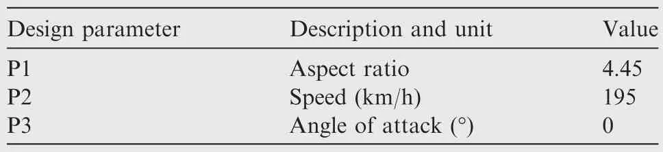
Table 2 Design parameters.

Fig.6 Geometric design variables in 3D model.

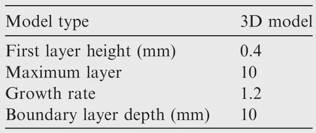
Table 3 Boundary layer specification.

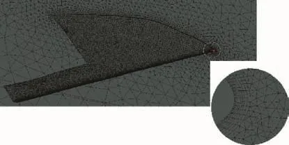
Fig.7 UAV mesh mapping and center plane cells in 3D model.

Fig.8 Grid convergence study.

Table 4 CFD solver properties.

Fig.9 DoE points distribution.

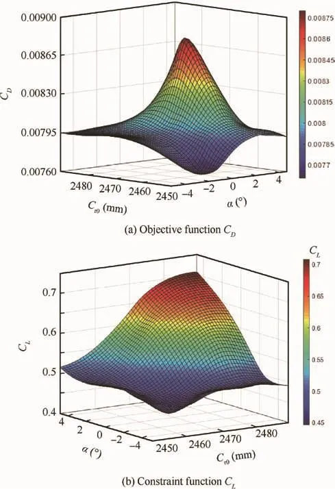
Fig.10 Meta-model built by Kriging method.

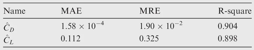
Table 5 Evaluation of constructed meta-mo dels.

Table 6 Optimal solutions of conventional aerodynamic shape optimization for BWB UAV.

In addition,the optimal point was evaluated in the highfidelity 3D model.The evaluation error guarantees the acceptability of the final result.The final shape of the BWB is shown in Fig.11.

Table 7 Optimal solutions for various initial points.

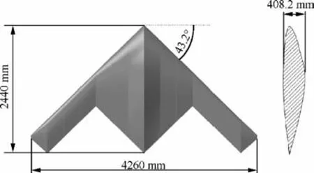
Fig.11 Conventional optimized blended wing body UAV dimensions.

3.2.Efficient aerodynamic shape optimization using multifidelity models for a BWB UAV

This section focuses on the implementation of the proposed framework of ‘efficient aerodynamic shape optimization” for the introduced samples.The aerodynamic optimization of the introduced BWB UAV is implemented step-by-step to show the impact of the methodology expressed in Section 2.The 3D model created in the earlier stage is used for deriving the low- fidelity model,extracting correction factors of the 2D model,and updating local meta-models in the optimization process.

3.2.1.2D geometry model

The 2D model with lower fidelity was created by selecting 15 sections of the UAV 3D model.In fact,airplane sections are analyzed in the airfoil 2D model using the panel method.As the BWB geometry is symmetrical,the sections were evaluated only in half of the UAV symmetry.Therefore,seven similar sections were deleted and the number reduced to eight.The first section was compatible with the UAV’s XOZ plane while other sections were parallel to it with an identical distance between them.The initial distance of the sections was 300 mm,which varies according to wingspan size during optimization.Fig.12 presents a view of the sections distributed in the 2D model.

The important point in modeling the low- fidelity model used in this article involves the variables related to wing length and sweep angle.The earlier works on wing and/or BWB UAV would overlook these variables to simplify optimization complexities if a low- fidelity model and/or a 2D model are used.56,57In these studies,only the 2D sections are analyzed and the result is generated regarding the entire BWB UAV.However,the effect of sweep angle on the performance and ultimate stability of a BWB,especially at high speeds,cannot be overlooked.58Therefore,it is expected that low- fidelity model cannot affect the accuracy of optimization results.

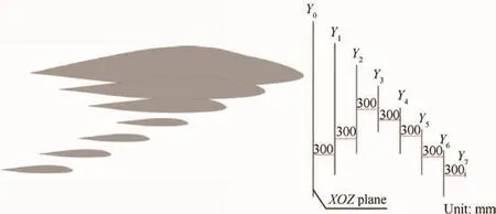
Fig.12 Section positioning in 2D model.

Fig.13 compares the analytical structure of a 3D model and a 2D model.The figure shows that the airplane structure is compared with the main model of the airplane in a 2D model(gray sections).It is clear that the lift and drag coefficients extracted from the 2D model differ from those of the main model and they have lower accuracies.However,the correction factor is determined as 0.85 for the 2D model after examining the differences in the analyses of the two models under similar conditions.

Based on investigation on 2D and 3D models(Figs.14–17),there are a number of minor differences between lift and drag correction factors,which are approximated to 0.85.

The coefficients CLand CDfor two-dimensional and three dimensional models are shown in Table 8.The coefficients CDand CLfor two-dimensional and three-dimensional models are shown in Fig.14.The ratio of the 3D drag coefficient to the 2D drag coefficient and the ratio of the 3D lift coefficient to the 2D lift coefficient are shown in Fig.15.

As shown in Fig.15(a),drag coefficient changes within the range of[0.82,0.865].Due to the range of 3D/2D drag ratio values,the correction factor is determined to be 0.85.As pointed in Fig.15(b),lift coefficient changes within the range of[0.84,0.86].Due to the range of 3D/2D lift ratio values,the correction factor is determined to be 0.85.

As explained above,the correction factor is determined as 0.85 for the 2D model after examining the differences in the analyses of the two models under similar conditions for lift and drag coefficients.

A total of 20 points are defined as variables in each section,whose airfoil varies by changing the specifications of the points in X and Z directions(Fig.16).Changing the angle of attack for each section also indicates a change in the angle of wing twist.

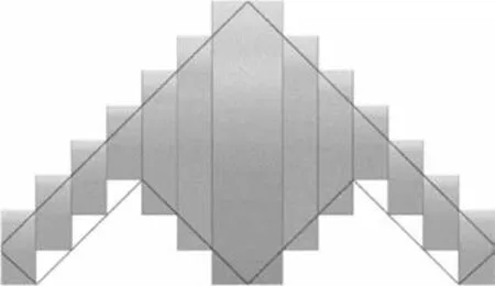
Fig. 13 Comparison between 2D and 3D model implementations.

Thus,327 variables are defined in this model,and changes in them would result in changes in their aerodynamic structures(Fig.6).A triangular grid provides further acceptable results for meshing such a 2D model(Fig.17).

This model evaluates mesh independence versus the number and dimensions of the elements.This examination is based on the diagram in one of the eight sections.The convergence shown by Fig.18 indicates the guarantee of accuracy for such a meshing.It should be noted that BWB’s CDis the result of drag coefficient in all sections.

Using the boundary layer specifications shown by Table 9,the model is prepared for the panel method.The constraints and solvers for analyzing the 2D model are selected completely similar to the 3D model(Table 4).Therefore,the comparison of the results obtained from the two optimization frameworks is valid.

As the 2D model is capable of conducting a high-speed analysis,it was used for extracting the initial design,determining dominant variables,and generating the initial global metamodel.

3.2.2.Constructing global meta-models

To specify the variables’effectiveness in drag coefficient reduction and increase the lift coefficient for deriving global metamodels,CFD solution of the low- fidelity model was collected for the 200 points obtained from uniform Latin hypercube strategy.

At this stage,the variables with the maximum effectiveness on aerodynamic coefficients were specified and other variables were deleted.ANOVA was performed on about 115 acceptable points obtained from this solution,showing that 25 variables in drag coefficient and 28 variables in changes of lift coefficient had maximum influence among 327 initial variables.Therefore,the initial variables were replaced by the effective variables.Comparison between the numbers and types of the selected variables and the dominant variables in the earlier optimization process not only indicates an accurate modeling of the 2D model but also promises an accurate optimization with shorter computational time.

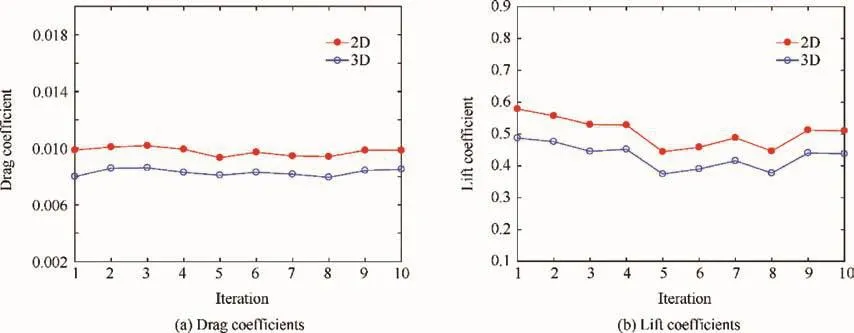
Fig.14 Drag coefficient and lift coefficient comparison for 2D and 3D models.

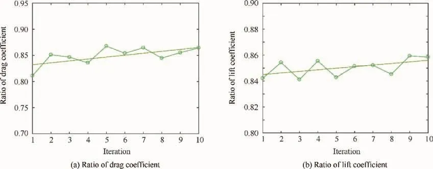
Fig.15 Ratio of 3D drag coefficient to 2D drag coefficient and 3D lift coefficient to 2D lift coefficient.

Fig.16 Shape design variable definition in an arbitrary section.

Fig.17 Meshing sections in 2D space.

The meta-models were then created from the feasible points for determining the values of lift and drag coefficients by utilizing Kriging method.Fig.19(a)shows the response of the extracted surface for objective function(CD)versus one of twist angles and chord length of the root section.Fig.19(b)shows the constraint(CL)response surface in proportion to one of the twist angles and the chord length of the middle section.As the figures highlight,the appropriate response was created in such a way that the effect of local extrema could be overlooked in the final shape and the global extrema would be the only option for optimization.

In addition,the accuracy and ability of the meta-models are verified(Table 10).The results indicate that the high efficiency of the optimization process is guaranteed due to the high accuracy of the meta-models.Therefore,the two frameworks are similar as far as the point selection and model creation method are concerned.

3.2.3.Implementing efficient aerodynamic shape optimization

At this stage,the meta-models are replaced with the aerodynamic model in the optimization framework.Fig.20 illustrates the differences between initial conceptual design and this point.The optimum point based on DoE is selected as the initial design point in the optimization process.

Optimization starts through the initialization of design variables and determination of their variation boundaries.The optimization process continues until the value of the optimal point becomes constant in two successive stages of the optimization.The termination criterion for optimization framework is defined as a difference smaller than 0.0001 between the optimal point and the initial point and/or an evaluation accuracy(Rs)greater than 0.998.This value is selected due to the reported accuracy in the studies conducted in this field.The acceptable value for evaluation error is the minimumvalues of Rsfor the objective function(CD)and the constraint function(CL).For instance,in the first stage,the Rsvalues for the objective function and constraint function are 0.965 and 0.95 respectively.Finally,the Rsvalue used in Eq.(9)min{0.965,0.95}=0.95.The maximum number of the selected iterations is seven with respect to the high accuracy of the meta-models(Table 10).In this case,there are six sample points in the first stages of optimization.

Table 8 Drag and lift coefficients for 2D and 3D models.

Fig.18 Grid convergence study in 2D section.

Table 9 Boundary layer properties in 2D model.

Fig.19 Initial global meta-model built by Kriging method.

Table 10 Evaluation of predictive capability of constructed meta-models.

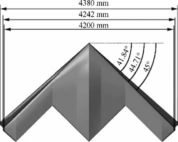
Fig.20 Initial design scheme versus initial conceptual design.

The need for updating is minimized due to a specific method for modeling the low- fidelity model,modifying it for a high overlap with the high- fidelity model,and specifically selecting the initial point of design.In other words,local modification of the meta-model is merely carried out in three iterations and the accuracy of the model is reported at an acceptable level with convergence to the optimal point.This shows the capability of the optimization algorithm to find the global optimal point.Otherwise,the meta-model has to be updated at any optimization iteration due to the major change in the optimal point neighborhood.

Finally,the cost function is fixed in the minimum value in the fourth iteration after three steps for updating the metamodels.Table 11 shows the data related to each stage of the optimization process.Stage 0 is selected as equal to the starting point of the design.Table 11 shows the mean variable boundaries.With the accuracy improving and variable bounds moving in the neighborhood of optimal point candidate,the mean of changes reduces quickly to make the convergence of response surface to the optimal point possible.

Table 12 shows the selected sample points at the different stages of optimization.In fact,both the number of sample points and its corresponding Rsconverge to 1.Undoubtedly,after some optimization iteration,the response surface around the optimal point becomes limited for finally being mapped to the optimal point.In this mode,the continuation of the optimization process is meaningless.

Table 11 shows that the optimal point found in the fourth iteration has a minimum drag coefficient as well as a greater lift coefficient.Comparison of Figs.5 and 21 reveals the final difference between the initial and optimized geometries.In spite of selecting the initial point near the optimal point and having an approximately fixed value for wingspan,the thickness and length of the chord of sections faced some changes.With respect to the relative changes of the values,the considerable difference in drag coefficient indicates the importance of geometric shape in the aerodynamicperformance of the UAV.This indicates the importance of optimization in this phase of aircraft design.

Table 11 Optimal solutions of efficient meta-model based aerodynamic shape optimization for BWB UAV.

Table 12 Number of sampling points and Rsin optimization process.

Fig.21 Optimized BWB UAV dimensions.

Another aspect of the proposed framework is its accuracy via the conventional method.Although the 3D model(highfidelity)is utilized in conventional strategy,updating lowfidelity RSM model based on 3D model and modifying variable bounds during optimization are recommended to improve framework capabilities,which will avoid unfeasible space and converge to optimal solution in minimum time without affecting accuracy,as shown in Tables 6 and 10.

Fig.22 shows the process of changing the UAV geometric model during the optimization process.While airfoil geometric changes are not noticeable at some points,some effective changes have been made at some points,especially in the trailing edge.This is true for any stage of optimization.As shown in Fig.22,some sections are subject to further changes at any stage of optimization.

With respect to the uncertain and unpredictable process concerning the deformation of sections,the changes finally lead to drag coefficient reduction.The option of a designer to achieve a proper optimal point in the optimization process is among the features of this method.In other words,with respect to the improvement of the accuracy of local models in each iteration related to the computational costs and time,the designer could continue or terminate the process.Moreover,the response surface is modified.However,it might not be the most optimal solution.As compared to the optimal solution found in the previous method,the result obtained from the proposed framework has altogether better performance.

Taking modeling time into account,the computational time of the proposed optimization method utilizing the high- fidelity model is approximately 3.5 h.Certainly,this period is much longer if the main model(high- fidelity model)is used,as seen in Table 13.

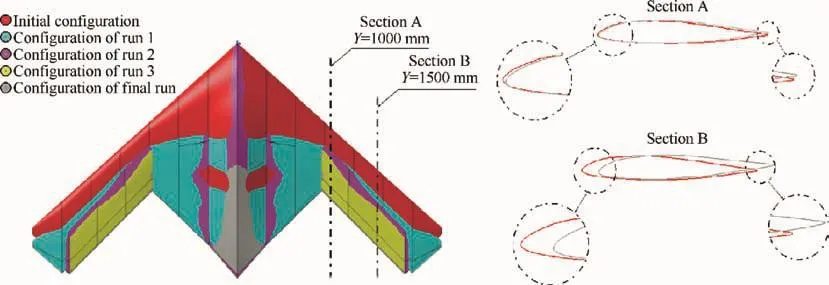
Fig.22 BWB geometric modification during efficient aerodynamic shape optimization using multi- fidelity models.

Table 13 Comparison of computational time between conventional and proposed aerodynamic optimization processes.

Of course,the final period extends to one day if the computational time for the pre-processing stage(creating the highfidelity model)is included.Table 13 shows the computational time for the proposed framework in the initial preparation and optimization stage as compared to the conventional optimization method.The considerable reduction of the computational time with no influence on solution accuracy exhibits the superiority of the proposed framework.

4.Conclusions

(1)The construction of the initial meta-models is based on the low- fidelity 2D panel model and the meta-models in the neighborhood of design point are locally modified based on the high- fidelity 3D CFD model in case of insufficient accuracy.

(2)As compared to creating an appropriate model using the high- fidelity model,the low- fidelity meta-model has much lower computational costs.Therefore,with respect to all the variables’effectiveness in the 2D model,modeling accuracy is improved considerably similar to the 3D model.

(3)The method’s major capability can be considered for those problems in which it is difficult to create a reliable meta-model in the whole design space.the points of strength of the presented framework is highlighted for those problems in which a designer selects fairly large variable boundaries for some reasons,such as inappropriate conceptual design and a lack of knowledge on the possible bound of the design optimal point.

(4)The proposed aerodynamic shape optimization framework based on multi- fidelity modelling is compared with the conventional aerodynamic shape optimization using high- fidelity(3D CFD)model and evaluated for a BWB benchmark case.Despite relatively low changes in the aerodynamic shape of sections and the overall dimensions of the aircraft,drag coefficient is reduced considerably.

(5)The comparative analysis between the results of the proposed and conventional approaches shows the absolute superiority of the proposed framework in terms of overall computational time.Meanwhile,the optimal design point obtained using the proposed approach clearly shows improvement in the accuracy of the results due to the compatibility of the local meta-model and customization of the appropriate design space.

1.Okonkwo P,Smith H.Review of evolving trends in blended wing body aircraft design.Prog Aerosp Sci 2016;82:1–23.

2.Wang Z,Huang W,Yan L.Multidisciplinary design optimization approach and its application to aerospace engineering.Chin Sci Bull 2014;59(36):5338–53.

3.Liu M,Hu Y.Robust design consideration in the multidisciplinary optimization of a flying wing UAV design.AIAA a erospace sciences meeting.Reston:AIAA;2014.

4.Boozer CM,Tooren MJL,Elham A.Multidisciplinary aerodynamic shape optimization of a composite blended wing body aircraft.AIAA/ASCE/AHS/ASC structures,structural dynamics,and materials conference.Reston:AIAA;2017.

5.Pan Y,Huang J,Li F,Yan C.Integrated design optimization of aerodynamic and stealthy performance for flying wing aircraft.Proceedings of the international multi conference of engineers and computer scientists;2017.

6.Morris A,Arendsen P,LaRocca G,Laban M,Voss R,Hon H.MOB—A European project on multidisciplinary design optimization.Proceedings of the international congress of the aeronautical sciences;2004.

7.Koziela S,Tesfahunegnc YA,Leifsson L.Expedited constrained multi-objective aerodynamic shape optimization by means of physics-based surrogates.Applied Mathematical Modelling 2016;40(15-16):7204–15.

8.Lyu Z,Martins JRRA.Aerodynamic design optimization studies of a blended-wing-body aircraft.J Aircraft 2014;51(5):1604–17.

9.Truong H,Zingg DW,Haimes R.Surface mesh movement algorithm for computer-aided-design-based aerodynamic shape optimization.AIAA J 2014;54(2):542–56.

10.Maruyama D,Liu D,Görtz S.An efficient aerodynamic shape optimization framework for robust design of airfoils using surrogate models.ECCOMAS congress 2016 on computational methods in applied sciences and engineering.2016 June 5-10;Crete Island,Greece:National Technical University of Athens;2016.

11.Hunsaker DF,Phillips WF,Joo JJ.Aerodynamic shape optimization of morphing wings at multiple flight conditions.AIAA aerospace sciences meeting.Reston:AIAA;2017.

12.Reist TA,Zingg DW.Aerodynamic design of blended-wing-body and lifting-fuselage aircraft.Proceedings of the AIAA applied aerodynamics conference.Reston:AIAA;2016.

13.Gan W,Zhou Z,Zhang X.Airframe-intake-exhaust integration design of flying wing using multi-bump strategy.Aerosp Eng 2016;231(13):2396–407.

14.Mader CA,Martins JRRA.Stability-constrained aerodynamic shape optimization of flying wings.Journal of Aircraft 2013;50(5):1431–49.

15.Lyu Z,Kenway GK,Martins J.RANS-based aerodynamic shape optimization investigations of the common research model wing.AIAA aerospace sciences meeting.Reston:AIAA;2014.

16.Li E,Wang H,Ye F.Two-level multi-surrogate assisted optimization method for high dimensional nonlinear problems.Appl Soft Comput 2016;46:26–36.

17.Paiva RM,Crawford C,Sul A.Robust and reliability-based design optimization framework for wing design.AIAA J 2014;52(4):711–24.

18.Rodríguez-Corts H,Arias-Montano A.Robust design optimization of a small flying wing planform based on evolutionary algorithms.The Aeronautical Journal 2012;116(1176):175–88.

19.Wang GG,Dong Z,Aitchison P.Adaptive response surface method–A global optimization scheme for approximation-based design problems.Eng Optim 2001;33(6):707–34.

20.Koziel S,Leifsson LT.Automated selection of low- fidelity models for rapid aerodynamic shape optimization using physics-based surrogates.AIAA/ASCE/AHS/ASC structures,structural dynamics,and materials conference.Reston:AIAA;2017.

21.Huang M,Yang X,Peng X.Efficient variable- fidelity multi-point aerodynamic shape optimization based on hierarchical kriging.AIAA aerospace sciences meeting.Reston:AIAA;2017.

22.Xia C,Tao Y,Jiang T,Chen W.Multi-objective shape optimization of a hypersonic lifting body using a correlation-based transition model.Aerosp Eng 2016;230(12):2220–32.

23.Yao W,Chen X,Huang Y,Michel MV.A surrogate based optimization method with RBF neural network enhanced by linear.Optim Methods Softw 2014;29(2):406–29.

24.Jones DR.A taxonomy of global optimization methods based on response surfaces.J Global Optim 2001;21:345–80.

25.Forrester AI,Keane AJ.Recent advances in surrogate-based optimization.Prog Aerosp Sci 2009;45(1–3):50–79.

26.Laurenceau J,Meaux M,Montagnac M,Sagaut P.Comparison of gradient-based and gradient-enhanced response-surface-based optimizers.AIAA J 2010;45(8):1–24.

27.Toal DJJ,Keane AJ.Efficient multi-point aerodynamic design optimization via co-kriging.J Aircraft 2011;48(5):1685–95.

28.Liu J,Song WP,Han ZH,Zhang Y.Efficient aerodynamic shape optimization of transonic wings using a parallel in filling strategy and surrogate models.Struct Multidiscip Optim 2016;55(3):925–43.

29.Wujek BA,Renaud JE,Batill SM.A concurrent engineering approach for multidisciplinary design in a distributed computing environment.Multidiscip Des Optim:Proc Appl Math Ser 1997;80:189–208.

30.Wujek BA,Renaud JE.New adaptive move-limit management strategy for approximate optimization,Part 1.AIAA J 1998;36(10):1911–21.

31.Pérez VM.Reduced-oder response surface approximations.In Homotopy-managed interior-point optimization [dissertation].Chicago:University of Notre Dame;2003.

32.Conn AR,Gould NIM,Toint PL.Trust region methods.Philadelphia:Society for Industrial and Applied Mathematics;2000.

33.Poole DJ,Allen CB,Rendall TCS.High- fidelity aerodynamic shape optimization using efficient orthogonal modal design variables with a constrained global optimizer.Comput Fluids 2017;143(17):1–15.

34.Ahmed MYM,Qin N.Surrogate-based aerodynamic design optimization:use of surrogates in aerodynamic design optimization.Proceedings of the aerospace sciences&aviation technolog.2009.

35.Nejat A,Mirzabeygi P,Panahi MS.Airfoil shape optimization using improved multiobjective territorial particle swarm algorithm with the objective of improving stall characteristics.Struct Multidiscip Optim 2014;49(6):953–67.

36.LyuZ,XuZ,Martin JRRA.Benchmarking optimization algorithms for wing aerodynamic design optimization.Proceedings of the international conference on computational fluid dynamics(ICCFD8);2014 July 14–18;Chengdu,Sichuan,China;2014.

37.Zhang M,Wang C,Rizzi A,Nangia R.Hybrid feedback design for subsonic and transonic airfoils and wings.AIAA aerospace sciences meeting.Reston:AIAA;2014.

38.Kuntawala NB.Aerodynamic shape optimization of a blendedwing-body aircraft configuration[dissertation].Toronto:University of Toronto;2011.

39.Ricco L,Rigoni E,Turco A.Smoothing spline ANOVA for variable screening.Dolomites Res Notes Approx 2013;6:130–9.

40.Taguchi G,Chowdhury S,Wu Y.Taguchi’s quality engineering handbook.New York:Wiley;2004.p.1736.

41.Hong HS,Hickernell FJ.Algorithm 823:Implementing scrambled digital sequences.ACM Trans Math Softw 2003;29(2):95–109.

42.Ye KQ,Li W,Sudjianto A.Algorithmic construction of optimal symmetric latin hypercube designs.StatPlann Inference 2000;90:145–59.

43.Myers RH,Montgomery A.Response surface methodology.Process and product optimization using designed experiments.New York:John Wiley and Sons;2001.

44.Breitkopf P,Naceur H,Rassineux A,Villon P.Moving least squares response surface approximation:formulation and metal forming applications.Comput Struct 2005;83(17–18):1411–28.

45.Ross TJ.Fuzzy logic engineering application.2nd ed.New York:John Wiley and Sons;2004.

46.Couckuyt I,Deschrijver D,Dhaene T.Fast calculation of multiobjective probability of improvement and expected improvement criteria for pareto optimization.Global Optim 2014;60(3):575–94.

47.McDonald DB,Grantham WJ,Tabor WL.Global and local optimization using radial basis function response surface models.Appl Math Model 2007;31:2095–110.

48.Persson J.Efficient optimization of complex products,a simulation and surrogate model based approach[dissertation].Linköping:Linköping University;2015.

49.Yaoa S,Guob D,Sunb Z,Yang G.A modified multi-objective sorting particle swarm optimization and its application to the design of the nose shape of a high-speed train.Eng Appl Comput Fluid Mech 2015;9(1):513–27.

50.Paiva RM,Carvalho ARD,Crawfordy C,Sulemanz A.A comparison of surrogate models in the framework of an MDO tool for wing design.Proceedings of the 50th AIAA/ASME/ASCE/AHS/ASC structures,structural dynamics,and materials conference.Reston:AIAA;2009.

51.Sivasubramani S,Swarup KS.Hybrid SOA-SQP algorithm for dynamic economic dispatch with valve-point effects.Energy 2010;35:5031–6.

52.Turco A.Adaptive filter SQP-description.Learning and intelligent optimization.Berlin Heidelberg:Springer;2010.p.68–81.

53.Turco A.Adaptive filter SQP-benchmark tests.ESTECO;2009.Report No.:Tec.Rep.2009–003.

54.Macconi M,Morini B,Porcelli M.Trust-region quadratic methods for nonlinear systems of mixed equalities and inequalities.Elsevier Sci Publ 2009;59(5):859–76.

55.Im J,Park J.Stochastic structural optimization using particle swarm optimization,surrogate models and Bayesian statistics.Chin J Aeronaut 2013;26(1):112–21.

56.Rashad R,Zingg DW.Aerodynamic shape optimization for natural laminar flow using a discrete-adjoint approach.AIAA Journal 2016;54(11).

57.Tesfahunegn YA,Koziel S,Gramanzini JR,Hosder S,Han ZH,Leifsson L.Application of direct and surrogate-based optimization to two-dimensional benchmark aerodynamic problems:A comparative study.AIAA aerospace sciences meeting.Reston:AIAA;2015.

58.Mader A,Martins JRRA.Optimal flying wings:a numerical optimization study.Proceedings of the AIAA/ASME/ASCE/AHS/ASC structures,structural dynamics and materials conference.Reston:AIAA;2012.