On Northern Hemisphere Wave Patterns Associated with Winter Rainfall Events in China

Claudia Christine STEPHAN,Yan Ho NG,and Nicholas P.KLINGAMAN

1 National Centre for Atmospheric Science–Climate,Department of Meteorology,University of Reading,Reading,RG6 6BB,United Kingdom

2 Department of Meteorology,University of Reading,Reading,RG6 6BB,United Kingdom

1.Introduction

The amount of precipitation over China during extended winter(November–April)is moderate compared to summer.Northerly winds associated with the East Asian winter monsoon transport dry and cold air from Siberia into China.Rainfall in this season usually benefits agriculture and hydropower plants.Nevertheless,winter extremes can be disruptive and costly when they involve blizzards,cold temperatures or flooding(Gao et al.,2008;Gu et al.,2008;Wang et al.,2008;Chang et al.,2011).

By applying empirical orthogonal teleconnection(EOT)analysis to observed 1982–2007 pentad rainfall anomalies,Stephan et al.(2017a)found that 43%of the intraseasonal rainfall variability in China during extended winter is explained by three spatial patterns of temporally coherent rainfall.The leading pattern(EOT-1)is centered along the Yangtze River and was associated with a wave train of Atlantic origin with significant anomalies two pentads in advance.Increased winter precipitation along the coast of Southeast China(EOT-2)was connected to an intensifying low pressure anomaly over Asia and wave propagation from the Mediterranean Sea.Intraseasonal rainfall variability between the Yangtze and Huaihe rivers(EOT-3)was associated with a quasi-stationary wave train that could be traced back to a strong anomalous ridge over northern Europe two pentads in advance.Stephan et al.(2017a)also performed an analogous analysis for summer.Summer patterns were predominantly associated with tropical convection instead of extratropical wave patterns.Therefore,this study focuses on winter.

Links between subseasonal weather extremes in China and extratropical disturbances have also been reported by others.Cold surges are associated with low air temperatures and strong winds in the midlatitudes and subtropics(Boyle and Chen,1987).Using empirical orthogonal function analysis of pentad precipitation data,Yao et al.(2015)found that the two dominant patterns of subseasonal precipitation variability in extended winter over China consist of a monopole in South China and a meridional dipole with opposite-signed precipitation anomalies over the Yangtze River basin and the southern coast.Yao et al.(2015)linked both patterns to a southward propagating cold surge,triggered by a wave train from the North Atlantic.In their composite analysis,Takaya and Nakamura(2005)also found the intraseasonal amplification of the Siberian high to be associated with a blocking ridge that is part of a quasi-stationary Rossby wave train propagating across the Eurasian continent.In a case study of the 2005/06 winter,Park et al.(2008)examined the causes of two consecutive cold surges.One was related to North Pacific upper-level blocking,and the other to an upper-level wave train across the Eurasian continent.Later,Park et al.(2011)grouped cold surges into “wave train”and “blocking”types based on circulation features,and discussed their relationship with the Arctic Oscillation(AO;Thompson and Wallace,1998).They found the blocking type was often associated with the negative AO phase,but no phase preference was found for the wave train type.Park et al.(2014)further examined the origins of the wave-train cold surge.At a lead time of approximately 12 days they reported negative upper tropospheric height anomalies southeast of Greenland;they suggested that these anomalies may originate in the lower stratosphere over the North Atlantic.Yao et al.(2015)and Stephan et al.(2017a)could not find evidence for stratospheric origins of precursor wave trains.

The above indicates that precursor circulations of winter rainfall events become statistically significant at lead times of approximately 10–12 days in regression or composite analyses.The physical nature of the wave trains and their origins remain unclear.Furthermore,previous research has not addressed whether it is possible to clearly identify these precursors for individual extreme events.If such precursors could be identified they could be used for an empirical prediction of rainfall extremes.Stephan et al.(2017a)and some of the other above-mentioned studies were based entirely on observations and reanalysis.In the present study,we repeat the Stephan et al.(2017a)EOT analysis on six simulations of the Met Office Unified Model(MetUM)Global Atmosphere 6.0 and Global Coupled 2.0 configurations at resolutions of∼200,90 and 40 km(in the zonal direction at the equator).This allows us to evaluate the model in terms of its ability to reproduce observed patterns of winter rainfall and to test the sensitivity of precursors to horizontal resolution and air–sea coupling.Secondly,by comparing synthetic time series to observations,we can assess the robustness of precursor circulations.

Section 2 introduces the simulations,data and methods.In section 3 we examine how well the simulations reproduce the observed EOT patterns.The observed and simulated precursors are compared in section 4.Individual events are discussed in section 5.Section 6 examines the dynamics of individual events.Section 7 addresses the wave origins and wave dynamics.A summary is given in section 8.

2.Data and methods

2.1.MetUM simulations

We analyze two 27-year atmosphere-only simulations of the MetUM Global Atmosphere configuration 6.0(GA6;Waltersetal.,2017)and four100-yearcoupled simulations of the Global Coupled configuration 2.0(GC2;Williams et al.,2015).If the model validates well,long simulations would provide synthetic catalogues of events longer than observations,for analysis of extremes and variability with a larger sample size.We refer to them as A96,A216,C96,C216,C512a and C512b,where“A”and“C”stand for“atmosphereonly”and “coupled”,respectively,followed by the nodal number(N96:1.875◦×1.25◦,208 km ×139 km in longitude and latitude at the equator;N216:0.83◦×0.55◦,93 km ×62 km;N512:0.35◦×0.23◦,39 km ×26 km).A96 and A216 use historical forcing;the GC2 simulations are present-day control simulations.Key information about the simulations is summarized in Table 1.A more detailed description of each simulation is given in Stephan et al.(2017b).

2.2.Observational data

Precipitation data are obtained from the Asian Precipitation–Highly Resolved Observational Data Integration Toward Evaluation of Water Resources(APHRODITE)dataset(Yatagai et al.,2012).This continental-scale daily product,from 1951–2007,with a resolution of 0.5◦×0.5◦,is produced from rain-gauge data after applying an objective quality control procedure(Hamada et al.,2011).We use 500 hPa geopotential height(Z500)for 1979–2007 from the European Centre for Medium-Range Weather Forecasts interim reanalysis(ERA-Interim;Dee et al.,2011).The resolution of these data is 0.7◦×0.7◦.Additional diagnostics are computed from ERA-Interim potential vorticity fields on isothermal surfaces and 200 hPa horizontal wind fields.For simplicity we refer to ERA-Interim as observations.

2.3.EOTs

The EOT analysis of 1951–2007 gridded APHRODITE precipitation data by Stephan et al.(2017a)serves as the ba-sis for this study.EOT analysis extracts spatial patterns of temporally coherent precipitation variability and returns time series that are mutually orthogonal(Smith,2004).Such variability is likely to have the greatest impact on infrastructure and human life due to its spatial organization.The steps of the algorithm are detailed in Stephan et al.(2017a).Before applying the technique to simulations,MetUM precipitation data are interpolated to the APHRODITE grid.We use linear regression onto EOT time series to link individual patternsto associated atmospheric precursors.To account for the non-Gaussian distribution of rainfall data,we use Spearman’s rank correlations to determine the statistical significance(always at the 10%significance level).

Table 1.Resolution,integration length and type of ocean coupling for all simulations.All simulations have 85 vertical levels with a model lid at 85 km.

2.4.Rossby wave source function

To diagnose the propagation of Rossby waves we compute the Rossby wave source(RWS)function as defined by Sardeshmukh and Hoskins(1988)in their Eq.(3).The 200 hPa absolute vorticity η,horizontal wind divergence D,and the divergent horizontal wind vector vvvχare combined to form

The first term describes divergence or convergence,respectively,above ascending or descending air,i.e.,the vorticity tendency arising from vortex stretching.The second term describes advection and becomes large where divergent wind encounters sharp horizontal vorticity gradients.The vertical pro file of the RWS peaks at 200 hPa because vorticity gradients associated with a vertical peak in the jet stream and divergent horizontal winds associated with convective out flow maximize at that level(Scaife et al.,2017).

2.5.Rossby wave ray tracing

We perform backward Rossby wave ray tracing to identify regions where waves may have originated.Given a slowly varying zonal flow with velocity U,the dispersion relation of a barotropic Rossby wave is

Here,ω is the frequency;k and l are the zonal and meridional wavenumbers,respectively;K=is the total wavenumber;and β∗= β −Uyyis the meridional gradient of the absolute vorticity of the mean flow,which combines the gradient in planetary vorticity β and the curvature of the flow Uyy,i.e.,the second meridional derivative of U(Hoskins and Karoly,1981).

For a stationary wave,ω=0,and Eq.(2)becomes

Hence,the zonal and meridional group velocities of a stationary wave are given by

and

respectively.To trace Rossby waves of a given zonal wavenumber k,we first compute l from Eq.(2).The previous location of the wave front is found from Eqs.(4)and(5),taking into account the spherical geometry of the globe.Points where U=0 form critical lines where the propagation of Rossby waves is not supported;the ray ends.A ray reverses its meridional propagation direction when l approaches zero and thus K2=k2.

The background wind Uis the November–Aprilmean climatological 200 hPa zonal wind.The background wind is smoothed using a 60◦zonal average.The curvature term Uyyis smoothed using a full 360◦zonal average.Our choices of pressure level,a two-hour time step,and smoothing of the background wind field,follow the recommendations in Scaife et al.(2017).They showed that rays are rather insensitive to the curvature term and time step,but that they are clearly affected by the choice of pressure level and the degree of smoothing of the background wind.We do not perform ray tracing on simulated wind data because 200 hPa wind biases are small and would not significantly alter rays.

2.6.Rossby wave initiation identification

Rossby wave initiation(RWI)segments are computed using the Ro¨thlisberger et al.(2016)algorithm.Ro¨thlisberger et al.(2016)discussed in detail the choice of the algorithm’s tuning parameters.We use their recommended parameters and here only briefly describe the algorithm.The algorithm extracts the geometry of isentropic 2 potential vorticity unit(PVU,1 PVU=10−6m2s−1K kg−1)contours,corresponding to the dynamical tropopause.For isentropic levels of 310–320 K(340–350 K),the contour is approximately aligned with the extratropical(subtropical)jet and can be used to measure its waviness(Hoskins et al.,1985;Martius et al.,2010).Every six hours and for 60◦longitudinal contour segments,starting every 3◦of longitude,the waviness d is measured by integrating the absolute latitudinal variations of the contour position over the length of the segment.Hence,a zonally aligned,straight jet corresponds to small d.The algorithm identifies wave-free segments(d<20◦)that show a strong increase(>8◦)in d within 30 hours.Candidate segments where increases in waviness may result from downstream development of existing waves are discarded if the waviness in one of the segments starting at 45◦longitude upstream of the candidate segment exceeds the waviness in the candidate segment by more than 4◦.

3.Fidelity of simulated EOT patterns

In the following we validate that MetUM GA6 and GC2 simulations accurately reproduce observed winter EOT patterns.To do so,simulated pentad precipitation is interpolated to the APHRODITE grid.We chose the APHRODITE grid so that the observed EOT patterns do not change from the ones reported in Stephan et al.(2017a).Then,for each simulation,China-wide precipitation is regressed against the simulated EOT time series.The same is done for APHRODITE.The resulting maps are shown in Figs.1–3.All MetUM simulations produce the precipitation associated with the three leading observed patterns(denoted Obs-1,Obs-2 and Obs-3),regardless of resolution or air–sea coupling.

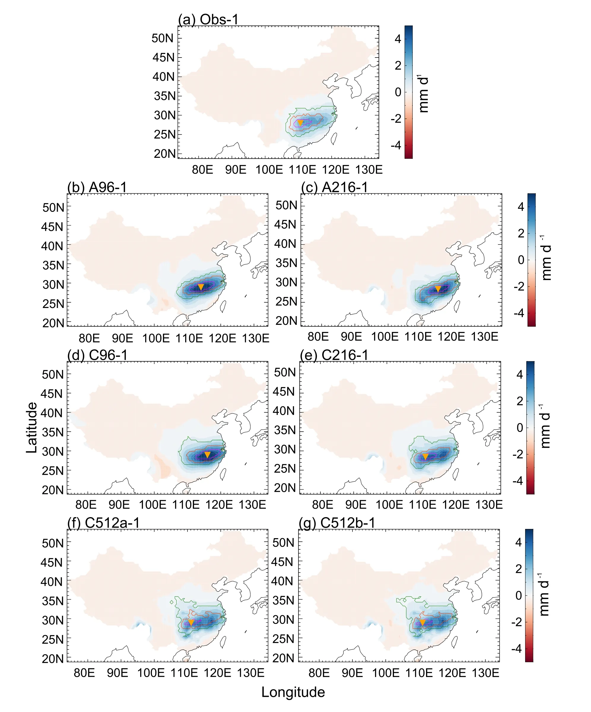
Fig.1.(a)Observed and(b–g)simulated EOT-1 patterns.Shading shows regressions of November–April precipitation against the normalized EOT time series.Also shown are correlations of the full precipitation-anomaly time series with the EOT base point exceeding 0.8(magenta),0.6(orange),and 0.4(green).The EOT base point is marked by the orange inverted triangle.

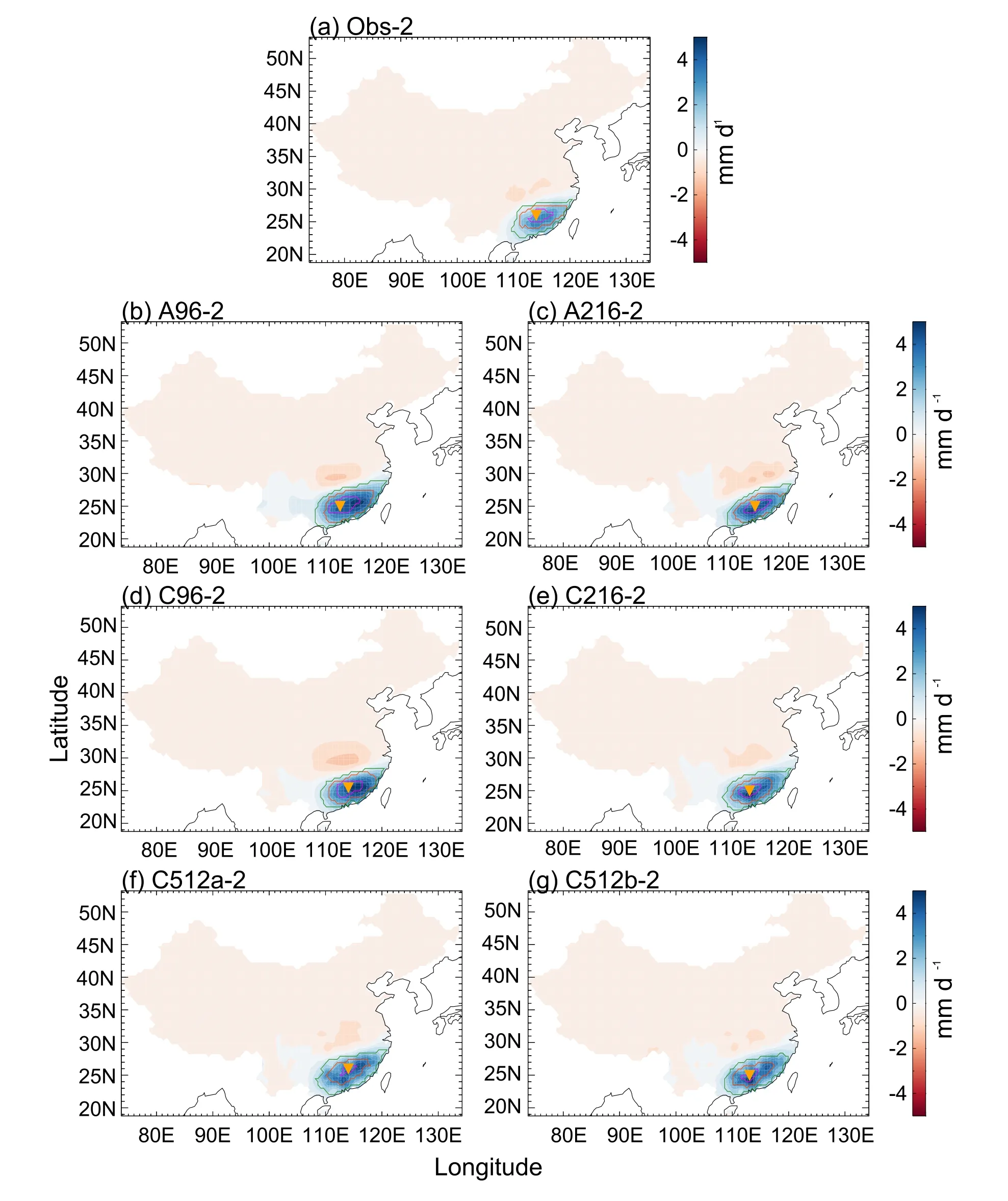
Fig.2.(a)Observed and(b–g)simulated EOT-2 patterns.Shading shows regressions of November–April precipitation against the normalized EOT time series.Also shown are correlations of the residual precipitation-anomaly time series with the EOT base point exceeding 0.8(magenta),0.6(orange),and 0.4(green).The EOT base point is marked by the orange inverted triangle.

Simulated rainfall anomalies match Obs-1,with pattern correlation coefficients exceeding 0.92(Table 2).The fraction of explained variance in the simulations(17%–25%)is close to the observed value(21%).The standard deviations of the simulated EOT time series are 25%–100%larger than in observations.This is consistent with positive biases in simulated intraseasonal variability and mean precipitation over Southeast China(not shown).Similar results are found for Obs-2(Fig.2).

Fig.3.(a)Observed and(b–g)simulated EOT-3 patterns.Shading shows regressions of November–April precipitation against the normalized EOT time series.Also shown are correlations of the residual precipitation-anomaly time series with the EOT base point exceeding 0.8(magenta),0.6(orange),and 0.4(green).The EOT base point is marked by the orange inverted triangle.

Obs-3 is situated further north(Fig.3),where biases in winter intraseasonal variability are small(not shown).Here,the simulated amplitude agrees with observations(Table 2).In the atmosphere-only simulations,A96 and A216,areas of covariability extend further northwest;in South China there is a large region with variability in the opposite phase.This explains why the fraction of explained variance for EOT-3 in A96 and A216 is higher(10%and 9%)than observed(7%).Pattern correlations exceed 0.67 for all simulations.

Table 2.Column 1:observed(Obs)and simulated(labeled by simulation name)EOT patterns in November–April;numbers indicate the order of the EOT pattern.Column 2:linear pattern correlation coefficient of simulated and observed precipitation anomalies.Column 3:explained spatiotemporal variance of the EOT pattern.Column 4:standard deviation of the EOT time series.

4.Precursors in regression analysis

Stephan et al.(2017a)described statistically significant circulation anomalies in regressions against EOT time series at lead times of up to two pentads(Tp=2;hereafter,Tpdenotes the lead time in pentads).These are reproduced in regressions of observed Z500and RWS at Tp=[3,2,1,0](Fig.4).Also shown are Z500regressions for C512a.Areas where all six MetUM simulations agree on the sign of the regression slope are shaded green.There is very good agreement in Z500anomalies between observations and all simulations.

Obs-1 is associated with high Z500over the eastern United States and central Europe,and low Z500over southern Greenland,northern Africa and Siberia at Tp=2.At Tp=1,there is a wavenumber-2 pattern of Z500anomalies between the North Atlantic and eastern Asia.At Tp=0,a zonal dipole is present over Asia and the western North Pacific.The RWS function indicates the genesis of upper tropospheric vorticity anomalies to the east of each of the above-mentioned Z500anomalies,indicating eastward propagation from the Atlantic sector through Europe to Asia.At Tp=3,observations show only small regions with significant Z500anomalies:high Z500over the northeastern US and the North Atlantic,and low Z500over southern Greenland.All simulations reproduce the Z500anomalies listed above and the anomalies are statistically significant,even at Tp=3.

Obs-2 is associated with low Z500in the Atlantic,northern Africa and South Asia,and high Z500over eastern Canada at Tp=3.At Tp=[2,1]there is low Z500over middle America,the Atlantic,and from northern Africa to South Asia,and high Z500at high latitudes between eastern Russia and eastern Canada and over western northern Africa.At Tp=0,there are two connected low Z500areas over the Middle East and East Asia.Prominent RWS anomalies are found in the Atlantic(Tp=3)and across northern Africa(Tp=[2,1]).Simulations produce the same low-latitude anomalies at Tp=[2,1,0].At Tp=3 they agree with observations on the low Z500in the Gulf of Mexico and the Atlantic.High Z500at high latitudes forms later in the simulations(Tp=1 instead of Tp=3),but so do the low Z500areas over northern Africa and South Asia(Tp=2 instead of Tp=3).This suggests that high-latitude anomalies develop in response to low-latitude anomalies,and that tropical anomalies are the relevant precursors of EOT-2 events in China.

Obs-3 is characterized by high Z500over northern Europe at Tp=[2,1,0].At Tp=[2,1],there is low Z500over northern Canada and Greenland.From Tp=2,low Z500areas also develop between northern Africa and Siberia,similar to Obs-1.A tripole of high Z500over northeastern Europe,low Z500over western Asia,and high Z500over East Asia,is present at Tp=[1,0].The strongest RWSs are found to the north of the Arabian Peninsula at Tp=1.All simulations agree on the development of the tripole at Tp=[2,1,0].Neither observations nor simulations show noteworthy anomalies at Tp=3.

The agreement between observed and simulated anomalies preceding precipitation associated with the leading three EOTs is remarkable and points to the existence of robust physical mechanisms or common statistical artifacts from regression analysis.Below we investigate whether the common anomalies discussed above may be used as potential predictors.

5.Impact of individual events

In February–March,eight of the ten strongest pentads in the APHRODITE EOT time series likely contributed to flooding,according to information provided by the Dartmouth Flood Observatory(http://floodobservatory.colorado.edu/). EOT-1 events#1,#8 and#9,and EOT-2 event#1,occurred simultaneously,with flooding during 15 March to 23 April 1992 in the provinces of Guangdong,Jiangxi,Fujian and Hunan.An area amounting to 200 000 ha was flooded,affecting 35 cities and counties,causing 248 casualties and 170 000 000 USD of damage.In addition,these EOT events occurred during the flooding in Guizhou and Sichuan during 15 March to 2 May 1992.Flooding,landslides and hailstorms injured 574,killed 59,and caused 70 000 000 USD of damage.EOT-1 event#2 and EOT-2 event#2 coincided with frontal storms and flooding in Hunan,Fujian,Changsa and Jiangxi during 6–13 March 1998.An area of 20 000 ha was flooded,130 people were displaced,and eight were killed.EOT-1 event#8 coincided with the Hong Kong flooding during 1 April to 8 May 1992.An April rainfall amount of 492.2 mm broke the record previously set in 1884.A total of 3000 people were displaced and five died.EOT-2 event#6 and EOT-3 event#10 were directly followed by flooding in Guangdong during 1–7 May 1993.The Beijiang River over flowed after 35 counties in the province received more than 100 mm of rain in the past week.The floods destroyed telecommunication facilities,power lines,dams and irrigation works,killed 65,displaced 3000,and caused damage amounting to 903 000 000 USD.Aside from the extratropical precursors identified by Stephan et al.(2017a)and examined further here,other large-scale drivers of precipitation variability,such as the El Niño–Southern Oscillation,and local processes,may have also contributed to the flooding.In any case,strong EOT events may exacerbate the risk of flooding.Therefore,it is necessary to examine the dynamics of individual events,rather than statistical composites alone.

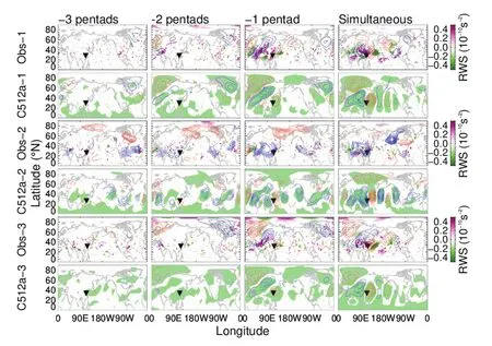
Fig.4.Observed and simulated Northern Hemisphere precursors of EOT events at lead times of 3–0pentads(left to right).Contours show Z500 regressed against the normalized observed and C512a EOT time series(blue,negative;orange,positive;intervals of 4 m for EOT-1 and EOT-3;1 m for EOT-2).The EOT base point is marked by the black inverted triangle.For observations,the regression of the RWS function(shading)is shown.All values are significant at the 90%confidence level.Green areas in the C512a panels show areas where all six simulations agree on the sign of the Z500 regression slope.

6.Precursors of individual events

Figures 5a–c show the percentage of the strongest positive 1/6 of EOT events that occurs during each month of extended winter.This climatology is computed by first finding the six strongest pentads in each November–April period(36 pentads),then aggregating over all years.Simulations generally reproduce the timing of top EOT events during the seasonal cycle,with the strongest events in February–March–April(FMA).To compare individual events between models and observations,we form a set of the 10 strongest EOT events in FMA(S10).Only including FMA events has the additional benefit of more consistent atmospheric background conditions.To avoid mixing EOT patterns,we constrain S10to only include pentads in which the amplitudes of the other two EOT time series do not exceed one standard deviation.S10does not include consecutive pentads.Normalized anomalies averaged over the region where correlations of the full(leading order)or residual(higher order)precipitation anomaly time series with the EOT base point exceed 0.5 are shown in Figs.5d–f.Observed and simulated S10anomalies are of comparable magnitude for EOT-1 and EOT-2.EOT-3 anomalies are greater in the simulations,because the 0.5 correlation region is larger in the simulations(Fig.3)and includes climatologically drier areas,where strong rainfall creates relatively larger percentage anomalies.

Fig.5.Characteristics of observed and simulated top EOT events.(a–c)Monthly occurrence of the top 1/6 EOT events.The color coding is the same as in(d–f).(d–f)Top 10 unmixed EOT events observed in FMA(S 10): five-day mean anomaly relative to the pentad climatology averaged over the area where correlations of the full(leading order)or residual(higher order)precipitation-anomaly time series with the EOT base point exceed 0.5.

All simulations capture the seasonality of top events and the magnitudes of S10sufficiently well for the purpose of comparing simulated and observed events and their precursors.Figures 6a–c show maps of precipitation anomalies averaged over S10.The black contour marks the region where correlations of the full or residual precipitation-anomaly time series with the EOT base point exceed 0.5.Consistent with the values in Figs.5d–f,rainfall anomalies inside this region are∼100%–300%.From the correlations shown in Figs.1–3,it is expected that the spatial distribution of rainfall differs from event to event.To measure the similarity of S10rainfall,Figs.6d–f show the number of events for which anomalies exceeded 100%.Inside the 0.5 correlation region,this number varies between 4 and 10 for EOT-1 and EOT-3;for EOT-2,it exceeds7 for most points.Thus,Figs.5d–fand Fig.6 show that S10contains a self-consistent sample of EOT events.Figure 6 was also computed for the six simulations to verify that their S10sets are self-consistent as well(not shown).The linear pattern correlation coefficients of Figs.6d–f and the corresponding maps for simulations vary between 0.26 and 0.52 for EOT-1,between 0.43 and 0.57 for EOT-2,and between 0.46 and 0.56 for EOT-3.In addition,we examined each event separately to confirm the consistency.

We next investigate similarities in the precursors associated with S10for EOT-1.Figures 7a–c are composites of observed Z500together with maps that show the number of events with Z500anomalies of the same sign.Z500anomalies are relative to 1982–2008 pentad climatologies.At Tp=2,we recognize several anomalies that are significant in the regression in Fig.4:high Z500over Scandinavia,and low Z500over northwestern Africa and Siberia and the North Atlantic.Except for the high Z500over Europe,these anomalies are seen in eight of ten events.At Tp=1,eight events agree on the tripolar Z500anomaly that extends from central Europe into the Arabian Sea.Mid-and high-latitude anomalies are shifted compared to the regression.In the simultaneous pentad,Z500anomalies are weak and differ greatly amongst S10.

The same information is given for C512a(Figs.7d–f)and C512b(Figs.7g–i).At Tp=2,nine or ten events in C512a exhibit low Z500to the west of Greenland and high Z500over northern Europe.The above-mentioned tripolar Z500low-latitude anomaly is also present in the composite at Tp=[2,1,0].Unlike observations,all C512a events show high Z500over the western North Pacific at Tp=0.C512b composites differ substantially from C512a.Similar to observations,they show only weak anomalies over the North Atlantic and Europe.However,C512b agrees on the low-latitude tripole at Tp=2 and all events exhibit a zonal dipole over Asia and the western North Pacific at Tp=0.We chose to show C512a and C512b because their 100-year long records allow us to best isolate strong and unmixed EOT events.Furthermore,their comparison lets us conclude that any agreement in C512a or C512b is not related to biases associated with the C512 configuration;instead,it is random.

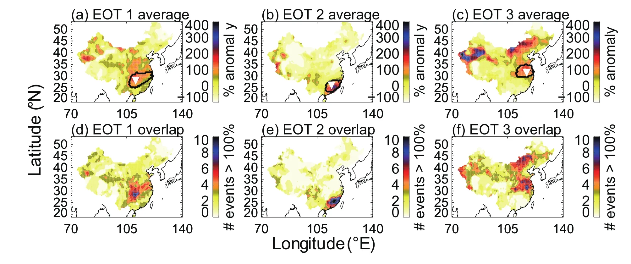
Fig.6.Precipitation characteristics of the top 10 unmixed EOT events observed in FMA(S 10).(a–c)Average five-day mean precipitation anomaly relative to the pentad climatology.The EOT base point is marked by the white inverted triangle.The black contour marks the region where correlations of the full(leading order)or residual(higher order)precipitation-anomaly time series with the EOT base point exceed 0.5.(d–f)Number of EOT events for which average five-day mean precipitation anomalies exceed 100%.

If we assumed that in each event and at each location negative and positive Z500anomalies occurred with equal likelihood,the chances that five,six,seven,eight,nine,and all 10 events agreed on the sign are 0.25,0.41,0.23,0.09,0.02 and<0.005,respectively.Averaged over observations,C512a and C512b,the fractions of grid points with this agreement are 0.25,0.42,0.23,0.08,0.02 and<0.005.This confirms that individual EOT-1 events show little agreement with the significant Z500anomalies of the regression.The dynamical evolution of the atmosphere is very different from event to event and does not resemble the slowly evolving or stationary features of the regression.From the comparison of observations,C512a and C512b,we conclude that there are no robust indicators of EOT-1 events that could serve as useful predictors at any lead time.These conclusions hold for the other four simulations and for EOT-2 and EOT-3.Aside from the Z500evolution,we also examined 200 hPa geopotential height,surface pressure,200 hPa wind,the AO(Thompson and Wallace,1998),North Atlantic Oscillation(Hurrell et al.,2003),Madden–Julian Oscillation(Madden and Julian,1972)and atmospheric blocking computed as in Henderson et al.(2016),but could not find significant or systematic indicators for any EOT.Despite this great inter-event variability,our set of MetUM simulations still accurately reproduces the observed EOT rainfall patterns and the observed Z500evolution for the overall regressions.Next,we consider whether there is a physical basis for this agreement.

7.Rossby wave dynamics

We investigate Rossby wave dynamics to explain the large inter-event variability in the atmospheric evolution preceding EOT events.Figure 8 shows the observed Z500regression for the three EOTs at different Tp.Dots mark Rossby wave rays every two hours.We perform backward tracing of rays that propagate into the target region(black box).Target regions are chosen to coincide with key local Z500anomalies at Tp=1.We choose Tp=1 instead of Tp=0 in order to limit the effect that latent heating may have on the Z500anomaly field.Rays are traced backwards for ten days or until they reach a region where propagation is not supported.The horizontal lines in Fig.8 mark 60◦-longitude RWI segments on the extratropical jet(blue)and the subtropical jet(red)that were observed within a given Tp.

At Tp=2,a pattern of high Z500in the North Pacific,low Z500over southern Greenland,and high Z500over central Europe is consistent with k=2 waves with possible origins in a broad region over the Pacific(Fig.8a).After 5–10 days they reach the Middle East and Asia,such that they may also contribute to the southwest–northeast tilted low Z500pattern at Tp=1,and to the high Z500over the Arabian Sea(the target region).The tripole between Europe and the Arabian Sea is consistent with k=3 propagation(Fig.8b).Note that these waves propagate from Europe to the Arabian Sea within only two to three days and could originate at various longitudes over the Atlantic basin.The EOT-2 target region represents the location of the eastern low Z500center in the regression at Tp=1.Rossby waves with k=3 may originate over Africa,central Europe or the North Atlantic(Fig.8c).All waves propagate across the western node of the low Z500anomaly.Frequent RWIs over Africa are consistent with the strong RWS anomaly in the regression.Recall that EOT-2 had statistically significant Z500and RWS anomalies over the Atlantic at Tp=3(Fig.4).The number of RWIs over the Atlantic is substantially higher than for the other EOTs(Fig.8d),providing further evidence that processes over the Atlantic may be influencing conditions over Africa in the following pentads.Low Z500over the target region is already present at Tp=3.Aside from the k=3 pathway,this may be communicated by k=1 waves originating over the western Atlantic(Fig.8d).

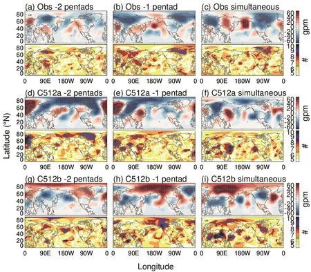
Fig.7.Inter-event variability in the evolution of Z500 for the top 10 unmixed EOT events in FMA(S 10)in(a–c)observations and(d–i)two simulations.The upper part of each panel shows the composite of Z500 at the designated lead time;the lower part shows the number of events where Z500 is of the same sign.

The EOT-3 target region extends from North China to Japan(Fig.8e).At Tp=2,Z500anomalies are well explained by k=1 waves.These contribute to the northern portion of the high Z500anomaly over the Barents Sea,the northern portion of the low Z500anomaly over Siberia,and the anomaly inside the target region itself.At Tp=1,k=2 waves with a large variety of origins are able to propagate into the target region.Possible source regions include the North Atlantic,the central North Pacific,the target region itself,eastern Russia,and North Africa.Given that all endpoints inside the target region are equally spaced in longitude and latitude and otherwise chosen at random,it is remarkable that all rays intersect significant Z500anomalies in these source regions(Fig.8f).These rays pass through the southern portion of high Z500over Europe,the central part of low Z500over Kazakhstan,and the high Z500in the target region.

The above shows that waves with different wave numbers and various origins pass through locations of convergent waveguides.These locations are associated with the strongest Z500anomalies in the regressions.Weaker Z500anomalies are found in locations that are less frequently crossed by waves associated with EOT events.Rather than coherent waves,the precursors in regressions are statistical amalgamations of more rapidly propagating waves with a variety of origins and properties.The 15–20-day timescale of precursors in regres-sion analysis is consistent with the period of low-frequency modulations and amplifications of alternating hemispheric flow regimes found in previous modeling and observational studies(e.g.,Wu,1993;Petoukhov et al.,2016).

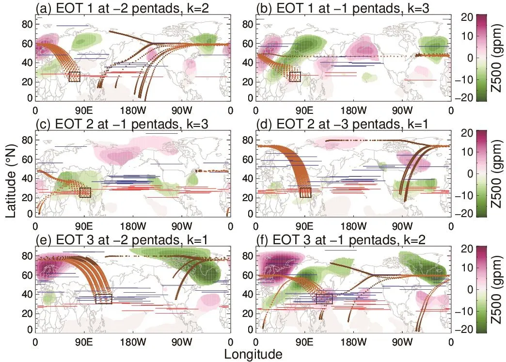
Fig.8.Wave dynamics preceding EOT events:regression of Z500 against normalized observed EOT time series(shading;significant at the 90%confidence level);60◦-longitude RWI segments(horizontal lines)on the extratropical(blue)and subtropical(red)jet for the top 100 unmixed EOT events;Rossby wave rays(dots)traced backwards in time from points inside the target region(black box)for 0–5 days(bright brown)and 5–10 days(dark brown).For unmixed EOT events,the considered EOT time series must exceed one standard deviation,while the other two EOT time series must have amplitudes smaller than one standard deviation.RWI segments are drawn at the mean latitude of the RWI segment.

8.Summary

In an EOT analysis of observed 1982–2007 pentad rainfall anomalies,Stephan et al.(2017a)found that 43%of the intraseasonal rainfall variability in China during extended winter is explained by three spatial patterns of temporally coherent rainfall.Using regression analysis,they connected this variability to extratropical wave disturbances with statistically significant precursors in Z500at lead times of approximately 10 days over Europe and the North Atlantic.Links between subseasonal weather extremes in China and extratropical disturbances have also been reported by other studies(Takaya and Nakamura,2005;Park et al.,2008,2011,2014;Yao et al.,2015).In regression or composite analysis,they also found statistically significant precursors at lead times of approximately 10–12 days.

Here,the aim was to better understand the dynamical evolution and the origins of the wave patterns found by Stephan et al.(2017a),to investigate whether precursors found in regression analysis may be used as predictors of strong extended winter rainfall events in China.We repeated the Stephan et al.(2017a)EOT analysis on six simulations of the MetUM,using atmosphere-only and coupled configurations at resolutions of∼200,90 and 40 km(in the zonal direction at the equator).There is excellent agreement in all simulations with the observed EOT patterns and precursor circulation anomalies.Hence,there is no evidence that the physical processes associated with EOT rainfall patterns are sensitive to air–sea coupling or to horizontal resolution.The robust simulation of extratropical wave disturbances would suggest the possibility for empirical prediction of EOT rainfall variability.However,in examining individual severe observed and simulated events,we found that the dynamical evolution of the atmosphere differs severely from event to event and does not resemble the slowly evolving or stationary features of the regression.In individual events,the most prominent anomalies in the regression can be missing,or of opposite sign.There are no robust indicators of EOT events that could serve as useful predictors at any lead time.Rossby wave dynamics are able to explain how the large inter-event variability is consistent with what appear to be slowly evolving orstationary waves.Using diagnostics based on observations and theoretical arguments,we showed that Rossby waves with a large variety of origins,wave numbers and group velocities can contribute to pressure anomalies over East Asia.Along their trajectories these waves produce common Z500anomalies that appear in composite or regression analysis as slowly evolving features.It is possible that this conclusion also holds for other extratropical teleconnection patterns.While anomalies in composite or regression analysis may not usefully predict rainfall,it is possible that EOT patterns are modulated in a predictable way by the slowly changing atmosphere–ocean coupled background state.Exploring this topic further could be an interesting avenue for future research.

Acknowledgements.Claudia C.STEPHAN was supported by the UK–China Research&Innovation Partnership Fund through the Met Office Climate Science for Service Partnership(CSSP)China,as part of the Newton Fund.Nicholas P.KLINGAMAN was supported by an Independent Research Fellowship from the UK Natural Environment Research Council(NE/L010976/1).APHRODITE data are available from http://www.chikyu.ac.jp/precip/.The RWS function was computed using code from the python package windspharm v1.5.0,available at http://ajdawson.github.io/windspharm.We thank Matthias R¨OTHLISBERGER for providing the Rossby wave initialization segment data and helpful discussions.

Open AccessThis article is distributed under the terms of the Creative Commons Attribution License which permits any use,distribution,and reproduction in any medium,provided the original author(s)and the source are credited.

REFERENCES

Boyle,J.S.,and T.J.Chen,1987:Synoptic aspects of the wintertime East Asian monsoon.Monsoon Meteorology,C.P.Chang,and T.N.Krishnamurti,Eds.,Oxford University Press,125–160.

Chang,C.P,Y.H.Ding,N.C.Lau,R.H.Johnson,B,Wang,T.Yasunari,2011:The Global Monsoon System:Research and Forecast.2nd ed.,World Scientific,43–72.

Dee,D.P.,and Coauthors,2011:The ERA-Interim reanalysis:Configuration and performance of the data assimilation system.Quart.J.Roy.Meteor.Soc.,137,553–597,https://doi.org/10.1002/qj.828.

Gao,H.,and Coauthors,2008:Analysis of the severe cold surge,ice-snow and frozen disasters in south China during January 2008:II.Possible climatic causes.Meteorological Monthly,34,101–106(in Chinese)

Gu,L.,K.Wei,and R.H.Huang,2008:Severe disaster of blizzard,freezing rain and low temperature in January 2008 in China and its association with the anomalies of East Asian monsoon system.Climatic and Environmental Research,13,405–418,https://doi.org/10.3878/j.issn.1006-9585.2008.04.06.(in Chinese)

Hamada,A.,O.Arakawa,and A.Yatagai,2011:An automated quality control method for daily rain-gauge data.Global Environmental Research,15,183–192.

Henderson,S.A.,E.D.Maloney,and E.A.Barnes,2016:The influence of the Madden-Julian Oscillation on northern hemisphere winter blocking.J.Climate,29,4597–4616,https://doi.org/10.1175/JCLI-D-15-0502.1.

Hoskins,B.J.,and D.J.Karoly,1981:The steady linear response of a spherical atmosphere to thermal and orographic forcing.J.Atmos.Sci.,38,1179–1196,https://doi.org/10.1175/1520-0469(1981)038<1179:TSLROA>2.0.CO;2.

Hoskins,B.J.,M.E.McIntyre,and A.W.Robertson,1985:On the use and significance of is entropic potential vorticity maps.Quart.J.Roy.Meteor.Soc.,111,877–946,https://doi.org/10.1002/qj.49711147002.

Hurrell,J.W.,Y.Kushnir,G.Ottersen,and M.Visbeck,2003:The North Atlantic oscillation:Climatic significance and environmental impact.Geophysical Monograph Series,134,279.

Madden,R.A.,and P.R.Julian,1972:Description of globalscale circulation cells in the tropics with a 40-50 day period.J.Atmos.Sci.,29,1109–1123,https://doi.org/10.1175/1520–0469(1972)029<1109:DOGSCC>2.0.CO;2.

Martius,O.,C.Schwierz,and H.C.Davies,2010:Tropopauselevel waveguides.J.Atmos.Sci.,67,866–879,https://doi.org/10.1175/2009JAS2995.1.

Park,T.W.,C.-H.Ho,and S.Yang,2011:Relationship between the Arctic Oscillation and cold surges over East Asia.J.Climate,24,68–83,https://doi.org/10.1175/2010jcli3529.1.

Park,T.W.,C.H.Ho,and Y.Deng,2014:A synoptic and dynamical characterization of wave-train and blocking cold surge over East Asia.Climate Dyn.,43,753–770,https://doi.org/10.1007/s00382-013-1817-6.

Park,T.W.,J.-H.Jeong,C.-H.Ho,and S.J.Kim,2008:Characteristics of atmospheric circulation associated with cold surge occurrences in East Asia:A case study during 2005/06 winter.Adv.Atmos.Sci.,25,791–804,https://doi.org/10.1007/s00376-008-0791-0.

Petoukhov,V.,S.Petri,S.Rahmstorf,D.Coumou,K.Kornhuber,and H.J.Schellnhuber,2016:Role of quasiresonant planetary wave dynamics in recent boreal spring-to-autumn extreme events.Proceedings of the National Academy of Sciences of the United States of America,113,6862–6867,https://doi.org/10.1073/pnas.1606300113.

R¨othlisberger,M.,O.Martius,and H.Wernli,2016:An algorithm for identifying the initiation of synoptic-scale Rossby waves on potential vorticity waveguides.Quart.J.Roy.Meteor.Soc.,142,889–900,https://doi.org/10.1002/qj.2690.

Sardeshmukh,P.D.,and B.J.Hoskins,1988:The generation of global rotational flow by steady idealized tropical divergence.J.Atmos.Sci.,45,1228–1251,https://doi.org/10.1175/1520-0469(1988)045<1228:TGOGRF>2.0.CO;2.

Scaife,A.A.,and Coauthors,2017:Tropical rainfall,Rossby waves and regional winter climate predictions.Quart.J.Roy.Meteor.Soc.,143,1–11,https://doi.org/10.1002/qj.2910.

Smith,I.,2004:An assessment of recent trends in Australian rainfall.Aust.Meteor.Mag.,53,163–173.

Stephan,C.C.,N.P.Klingaman,P.L.Vidale,A.G.Turner,M.-E.Demory,and L.Guo,2017a:A comprehensive analysis of coherent rainfall patterns in China and potential drivers.PartII:Intraseasonal variability.Climate Dyn.,https://doi.org/10.1007/s00382-017-3904-6.(in press)

Stephan,C.C.,N.P.Klingaman,P.L.Vidale,A.G.Turner,M.-E.Demory,and L.Guo,2017b:Interannual rainfall variability over China in the MetUM GA6 and GC2 configurations.Geo-scientific Model Development,https://doi.org/10.5194/gmd-2017-252.(in press)

Takaya,K.,and H.Nakamura,2005:Mechanisms of intraseasonal amplification of the cold Siberian high.J.Atmos.Sci.,62,4423–4440,https://doi.org/10.1175/JAS3629.1.

Thompson,D.W.J.,and J.M.Wallace,1998:The Arctic oscillation signature in the wintertime geopotential height and temperature fields.Geophys.Res.Lett.,25,1297–1300,https://doi.org/10.1029/98GL00950.

Walters,D.,and Coauthors,2017:The met Office unified model global atmosphere 6.0/6.1 and JULES global land 6.0/6.1 configurations.Geoscientific Model Development,10,1487–1520,https://doi.org/10.5194/gmd-10-1487-2017.

Wang,L.,and Coauthors,2008:Analysis of the severe cold surge,ice-snow and frozen disasters in south China during January 2008:I.Climatic features and its impact.Meteorological Monthly,34,95–100.(in Chinese)

Williams,K.D.,and Coauthors,2015:The Met Office Global Coupled model 2.0(GC2)configuration.Geoscientific Model Development,8,1509–1524,https://doi.org/10.5194/gmd-8-1509-2015.

Wu,P.,1993:Nonlinear resonance and instability of planetary waves and low-frequency variability in the atmosphere.J.Atmos.Sci.,50,3590–3607,https://doi.org/10.1175/1520-0469(1993)050<3590:NRAIOP>2.0.CO;2.

Yao,Y.H.,H.Lin,and Q.G.Wu,2015:Subseasonal variability of precipitation in China during boreal winter.J.Climate,28,6548–6559,https://doi.org/10.1175/JCLI-D-15-0033.1.

Yatagai,A.,K.Kamiguchi,O.Arakawa,A.Hamada,N.Yasutomi,and A.Kitoh,2012:APHRODITE:Constructing a long-term daily gridded precipitation dataset for Asia based on a dense network of rain gauges.Bull.Amer.Meteor.Soc.,93,1401–1415,https://doi.org/10.1175/BAMS-D-11-00122.1.