ENSO Predictions in an Intermediate Coupled Model In fluenced by Removing Initial Condition Errors in Sensitive Areas:A Target Observation Perspective

Ling-Jiang TAO,Chuan GAO,and Rong-Hua ZHANG∗,3

1Key Laboratory of Ocean Circulation and Waves,Institute of Oceanology,Chinese Academy of Sciences,Qingdao 266071,China

2University of Chinese Academy of Sciences,Beijing 100029,China

3Qingdao National Laboratory for Marine Science and Technology,Qingdao 266237,China

1.Introduction

El Ni˜no–Southern Oscillation(ENSO)is an ocean–atmosphere coupled phenomenon involving anomalous warming or cooling in the central and eastern tropical Pacific(Philander,1983).It has been much focused upon by scientists and the general public because of its effects on natural disasters around the world(King,1997).In recent decades,continued intensive studies of El Ni˜no events have promoted its simulation and prediction(Zebiak and Cane,1987;Latif et al.,1993a;Tang,2002;Tang and Hsieh,2002;Zhang et al.,2003,2005b).However,signi ficant uncertainties still exist in real-time ENSO prediction(Latif et al.,1993b;Chenand Cane,2008).Particularly,most ENSO models tend to be less predictable when predictions are made before or during the northern spring(Zebiak and Cane,1987;Webster,1995;Fl¨ugel and Chang,1998;Fan et al.,2000;Zhang et al.,2005b).Such a seasonally dependent phenomenon is referred to as the “spring predictability barrier”(SPB),which is considered one of the main factors limiting ENSO prediction skill.

Observations are fundamental for understanding ENSO-related dynamics,developing numerical models and improving prediction skill.Recently,a 10-year international program,called TOGA(Tropical Ocean–Global Atmosphere),was carried out to monitor the tropical ocean in real time.The program yielded many great successes.Particularly,an ENSO observing system has been established,including the Tropical Atmosphere Ocean(TAO)/Triangle Trans-Ocean Buoy Network(TRITON)array,which has been a major part of the Global Ocean Observing System(McPhaden et al.,1998).Further,with the implementation of the Argo(Array for Real-time Geostrophic Oceanography)plan(Feder,2000),a growing number of international organizations have released Argo floats into the global ocean.Thus,real-time observations of temperature,salinity,density and currents in the global upper ocean are available.So far,these observ-ing systems have been able to offer large quantities of observational data(especially subsurface ocean data),which have greatly promoted our understanding of the ocean,atmosphere,and their interactions.However,the spatiotemporal sampling frequencies of present observational strategies are obviously insufficient.Meanwhile,ENSO processes are known to be strongly regionally dependent.As a result,initial states in some areas can be more important than others in terms of ENSO predictions.Such areas are the so-called“sensitive areas”or “key areas”(Mu et al.,2015).Making use of observations in sensitive areas can have larger effects on prediction performance than other areas.It can be noted that as more and more buoys of the TAO/TRITON array have collapsed in recent years,it is quite urgent to redesign a new and reasonable observation network,particularly regarding high-impact ocean–atmosphere environmental events(such as ENSO).Additionally,considering the high cost of ocean observations, finding sensitive areas to maximize prediction skill is economically necessary.

Therefore,a key issue is how to identify sensitive areas.Many mathematical techniques have been developed to determine these regions,including the singular vector(SV)approach(Palmer et al.,1998),the ensemble transform technique(Bishop and Toth,1999),adjoint-derived sensitivity(Wu et al.,2007),and the ensemble transform Kalman filter(Bishop et al.,2001).Such a strategy to find sensitive regions where intensive observations are optimally implemented for maximizing prediction improvements is the so-called“target observation”or“adaptive observation”method.

Mu et al.(2003)extended the SV method and proposed the so-called conditional nonlinear optimal perturbation(CNOP)technique,which has also been widely used in target observations of high-impact climate events(Zhu and Thorpe,2006;Mu et al.,2009;Yu et al.,2012;Duan and Hu,2016).Based on a theoretical ENSO model(Wang and Fang,1996),Mu et al.(2003,2007a)demonstrated that the initial error growth induced by CNOPs tends to be larger than that by the SV approach.Yu et al.(2009)studied the horizontal distributions of CNOPs in the Zebiak–Cane(ZC)model(Zebiak and Cane,1987),and identified two types of CNOPs that can induce the largest uncertainties in El Ni˜no prediction.Duan and Wei(2013)demonstrated the existence of CNOP-like errors in realistic ENSO predictions,which,together with the results of Yu et al.(2012),suggests that a reduction in the CNOP-like error components in initial conditions could provide an effective way to improve ENSO prediction skill.In addition,some studies have revealed that observations in CNOP-indicated sensitive areas not only can improve the quality of initial conditions,but also better detect the early signals of El Ni˜no events(Mu et al.,2014;Hu and Duan,2016).

Due to the varying complexity of models,sensitive areas identified for ENSO predictions may appear somewhat different.For example,based on a relatively complicated model,the Community Earth System Model(CESM),Duan and Hu(2016),in addition to the eastern Pacific,further emphasized the role of the subsurface state.Based on CMIP5 model outputs,Zhang et al.(2015)suggested that sensitive areas are located in the central-eastern equatorial surface region and eastern tropical subsurface region.Conversely,Kumar et al.(2014)showed that observing in the central Pacific is more important than in the eastern Pacific because the former region is of foremost importance in preserving the “memory”of ENSO evolution.Penland and Matrosova(1994)also suggested that the central equatorial Pacific,close to the date line,is of great importance in El Ni˜no evolution.

Previously,Zhangetal.(2003)developed a relatively new intermediate coupled model(ICM).The ICM(IOCAS ICM,named after the Institute of Oceanology,Chinese Academy of Sciences)is an ENSO model that has been routinely used for real-time predictions and whose results are collected at the International Research Institute for Climate and Society,Columbia University.An obvious high prediction skill is found in the central equatorial Pacific[e.g.,the correlation coefficient is about 0.7 with a six-month lead time;refer to Zhang et al.(2005b,see their Fig.12)],so the ICM can predict the SST anomalies in the Ni˜no3.4 area well.In addition,this ICM has been widely used for ENSO modeling(Zhang et al.,2005a,2008,2013;Gao and Zhang,2017;Gao et al.,2017).Recently,Gao et al.(2016)implemented a four-dimensional variational(4DVar)data assimilation method into the ICM,which provides optimized initial conditions so that the prediction skill of ENSO events is improved efficiently.Besides,the 4DVar-related adjoint component of the ICM provides technical support to exploit the CNOP method.Tao et al.(2017)performed CNOP-based analyses using the ICM and identified the CNOP-type initial errors in the SST and sea level(SL)that can in duce the largest error growth in El Ni˜no predictions.It was found that the identified CNOPs are significantly dependent on the initial times.Furthermore,the CNOP-induced error evolutions are strongly season-dependent,which is known as the SPB phenomenon.Therefore,Tao et al.(2017)suggested that seasonally varying target observations(particularly,deploying observations in the central and eastern equatorial Pacific)could profoundly weaken the SPB phenomenon and thus significantly improve the ENSO prediction skill.However,Tao et al.(2017)did not explore the extent to which removing initial condition errors in the CNOP-determined sensitive areas can have an effect on the prediction skill.Also,it is not known whether CNOP-related target observations are advantageous to reducing the SPB phenomenon in prediction experiments.

Accordingly,in the present study,ideal observing system simulation experiments(OSSEs)are performed using the ICM to demonstrate the extent to which El Ni˜no predictions can be improved by removing initial condition errors in various target areas.First,a simulated ENSO event is chosen as the “true”event.Then,control prediction experiments are performed in which errors are added into the “true”initial stat es in the tropical Pacific.Finally,targe to bservation experiments are performed in which the initial condition errors are removed in a certain area.Such experiments serve to identify the sensitive areas for ENSO predictions.In addition,various target observation experiments with combinations of these subregions are further performed to verify whether the CNOP-determined areas are important for ENSO predictions.

Following this introduction,the ICM and the idealized OSSEs are described in section 2.Then,the results from the control prediction experiments are reported in section 3,followed by discussion in section 4 on the importance of observing in different areas in the tropical Pacific.In section 5,the results from the CNOP-related target observation experiments are presented.And finally,the study’s main conclusions and some further discussion are provided in section 6 and section 7,respectively.

2.Experimental design

This section briefly reviews the ENSO model used and the prediction experiments in terms of the OSSE strategy.These methods and numerical model are used to explore the extent to which ENSO prediction skill can be improved by removing initial condition errors in some sensitive areas,which are identified by the CNOP approach.

2.1.Model description

As illustrated in Fig.1,the ICM,developed by Zhang et al.(2003),includes a statistical atmosphere submodel(i.e.,τ model),an intermediate dynamic ocean model(IOM),and an SST anomaly submodel embedded with an empiricalTesubmodel for representing the temperature of subsurface water entrained into the mixed layer(Te).

The dynamical ocean part of the ICM was established by Keenly side and Klee man(2002),andincludeslinearandnonlinear dynamical components.The linear component is derived from the baroclinic model of McCreary(1981),but was extended to have a horizontally varying background strati fication.The first 10 baroclinic modes are retained in the vertical layers,while two surface layers determined by Ekman dynamics include the combined effect of higher baroclinic modes from 11 to 30.The nonlinear component is added into the two surface layers as a correction to the linear component so that the neglected nonlinearity is considered.As a result,the IOM can simulate the ocean currents well.Further details regarding the IOM can be found in Keenlyside and Kleeman(2002).

A fully nonlinear SST anomaly submodel is implemented into the dynamic ocean model to describe the thermodynamics for the surface mixed layer.The tendency of the SST anomaly is determined by horizontal and vertical advection,thermal diffusion and thermal dissipation.Note that dynamic processes play a pivotal role in regulating the SST in the cold tongue region of the tropical Pacific.Therefore,the processes associated with subsurface water entrained into the surface(i.e.,Te)should be dealt with carefully.Extensive studies have shown that there is a strong correlation between SL andTevariability(Zhang et al.,2004;Kumar et al.,2014).Thus,an empiricalTesubmodel is constructed based on the SVD method(Zhang et al.,2005b).TheTesubmodel is determined involving two steps: first,an inverse modeling ofTeis used to determine the optimized historicalTewhen providing the other terms of the SST equation,such as the observed SST and velocity fields;and second,a relationship between SL andTeis determined by the SVD analysis from the historicalTeand SL data.Then,aTeanomaly can be obtained from a given SL anomaly,which is used for the SST anomaly equation.

Similar to theTesubmodel,an atmosphere submodel is also constructed based on the SVD analysis,which is used to only represent the wind stress(τ)interannual anomaly.The relationship between the historical τ anomaly and SST anomaly is determined by SVD analysis,which is used to determine the τ anomaly from the SST anomaly.The various datasets used in the ICM are detailed in Zhang et al.(2005b).

These three submodels constitute a coupled model that includes wind-driven ocean dynamics and thermodynamics in the upper ocean.As shown in Fig.2,the ICM can successfully simulate the dominant four-year oscillation period of interannual variability and phase locking associated with ENSO cycles.

2.2.Idealized OSSEs

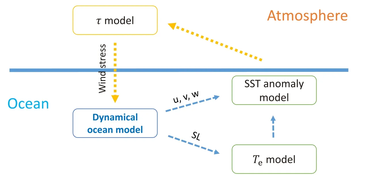
Fig.1.Schematic illustration of the ICM,consisting of a dynamical ocean model,statistical atmosphere model,and SST anomaly model with an empirical Teparameterization.

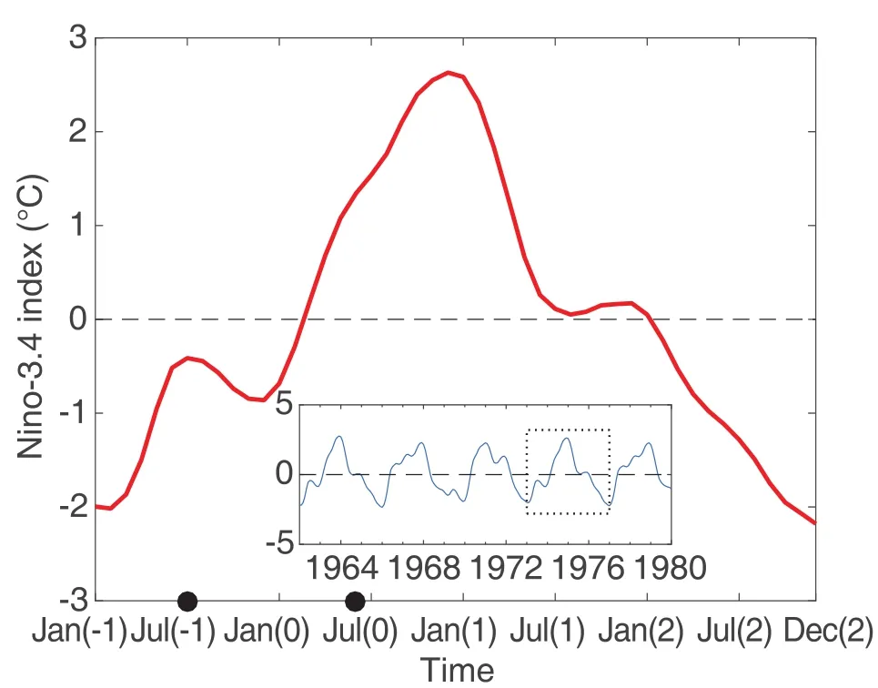
Fig.2.Time series of Ni˜no3.4 indices(units:°C)simulated by the ICM.Note that since stochastic processes are excluded in the ICM,the depicted ENSO is regular with a four-year period;see the plotted Nino3.4 index,which is partly displayed in the embedded panel.One simulated ENSO cycle(red line),also framed by the dashed border,is chosen as a “true”state,which is used as a reference when making prediction experiments with various target observation strategies.The months marked by the black points during the periods from Jul(−1)to Jun(0)are the start months from which predictions are made.

OSSEs have been widely used to evaluate the importance of different observational networks for climate/weather predictions(Lord et al.,1997;Morss and Battisti,2004a,2004b;Lee et al.,2016).In the context of classical OSSEs,a long free model run is first used to generate the“truth”evolution of the climate system(denoted as the “true”run).Then,realistic errors are artificially added into the “true”run fields as observations for all observing systems.Finally,a predictive model that derives from the“true”run model but with introduced model errors is used to perform predictions based on a range of observing system and data assimilation techniques,and compared with the “true”run to identify the optimal observing system and also quantify its improvements.More details on OSSEs can be found in Masutani et al.(2010).Because the observations formed in the OSSEs are identified from a numerical model in which initial conditions and the evolution of ENSO can be determined,various observational networks can be redesigned optionally.Therefore,OSSEs become an effective method for target observation.

In the present study,OSSEs are adopted in an idealized situation.In the idealized OSSEs,the initial condition errors are directly removed instead of performing complicated data assimilations in the observing regions,and the model errors are ignored(i.e.,the predictive model is identical to the“true”model run).In additional to the“true”El Ni˜no event run from the ICM,the idealized OSSEs include two prediction experiments(or runs):one serves as a control prediction experiment in which predictions are made using the initial conditions from the “true”ENSO case,with errors being added in the whole tropical Pacific;and the other,called the target observation experiment,involves the initial condition errors that formed in the control prediction experiment being removed in the observing region.The idealized OSSEs can fully demonstrate the potential of target observations to improve the ENSO prediction skill.In some cases,the idealized OSSEs are similar to the so-called “identical twin”experiments.

2.2.1.A“true”event

2.2.2.Control prediction experiments

Next,we perform control prediction experiments in which predictions are made using the initial conditions derived from the “true”state with added errors.Accordingly,the predicted SST anomaly is deviated from the “true”ENSO event.Note that the prediction models can be generally initialized by data assimilations or taken from reanalysis data;therefore,the initial errors tend to have a certain structure rather than a simple random distribution in the realistic prediction.A key issue,then,is how to construct the initial condition errors.

Based on hindcast experiments,Duan et al.(2009)recently proposed an ensemble-based algorithm to construct the initial condition errors and explored the SPB-related initial condition errors using the ZC model.Later,Duan and Hu(2016)implemented the ensemble-based algorithm to investigate the SPB-related initial errors with a relatively complicated model(namely,CESM).Such ensemble-determined error fields are highly responsible for many ergodic initial errors with certain structures.In this study,we use the same method to construct the error fields using the ICM.The main con figurations are as follows:

For consistency with Tao et al.(2017),the initial errors consist of two components:the SST and SL anomaly fields.The initial error fields are then generated by taking the differences between the SST/SL anomalies of the“true”El Ni˜no state in the start month and that in each month of the four years preceding the start month.For example,when making predictions from January(0),the first member of initial errors in the SST/SL anomalies are obtained by subtracting the SST/SL in December(−1)from that in January(0);when taking the differences in SST/SL between November(−1)and January(0),we can obtain the second member of errors in the initial conditions,and so on.Considering the effect of a large SPB on onset-phase prediction(Tao et al.,2017),we focus on the start time from July(−1)to June(1).Then,48×12 error fields can be obtained for 12 start months,each having 48 types of errors that will be added into the corresponding initial“true”state to perform a 12-month prediction.Consequently,48 kinds of time series for the predicted SST anomalies are obtained at each start month.Note that the numerical models are supposed to be perfect.Thus,the ICM used to perform prediction experiments for the El Ni˜no event has the same con figuration(such as the model parameters)as the“true”run.

2.2.3.Target observation experiments

To find the most effective areas where the observations have a dominant role in El Nino predictions,we perform target observation experiments,which are the main part of OSSEs.The tropical Pacific(30°N–30°S,120°E–80°W)is equally divided into 12 subregions(Fig.3;each subregion is referred to as S1,S2,etc.)as target areas.To represent observing in one certain area(i.e.,one subregion),we remove the initial condition errors(which are formed from the control prediction experiments)in the corresponding target area when initializing the prediction.Then,we can evaluate the extent to which the maximum effect can influence the prediction skill by comparing the results from the control prediction experiments and the target observation experiments.Based on these 12 subregions,12 prediction experiments are carried out with the initial errors in the corresponding target areas being removed.For example,the S1 target observation experiments are considered to investigate the effects induced by target area S1 when the initial condition errors are removed in the S1 area,and the model is then integrated over 12 months from the start time of July(−1)to June(0).Then,12 sets of idealized prediction experiments(hereafter referred to as target observation experiments S1–12)are performed with corrected initial conditions in the target areas.Through comparison with the predicted results from the control prediction experiments,we can evaluate the efficiency of the initial conditions through the target observation strategy for El Ni˜no predictions.

Experiments indicate that simply removing initial condition errors in one target area may worsen the prediction due to the opposite effects of initial errors in other regions(Yu et al.,2012),which may also be due to the imbalance of initial fields.Thus,we perform the target observation experiments by combining multiple areas together.That is,target observation experiments are conducted simultaneously in multiple areas.Various combinations of target observation experiments are conducted in advance.Then,several effective observational networks are identi fied in terms of their effects on El Nin˜o predictions.More details on the target observation experiments are provided in Table 1.The results are given based on the TA26,TA68,TA268,TA1256 and TA5678 observational networks.Taking the TA26 observational network as an example,the prediction model is initialized by removing the initial condition errors in both the S2 and S6 areas.Note that Tao et al.(2017)showed that sensitive areas for ENSO predictions in the ICM are located in the central and eastern Pacific(Tao et al.,2017,Fig.4).Those observational networks(i.e.,multi-area observation strategies,such as TA26,TA68,etc.)are closely related to the CNOP-determined areas(a replica of CNOP is shown in Fig.3).Thus,such observation experiments are renamed as CNOP-related target observation experiments for convenience.

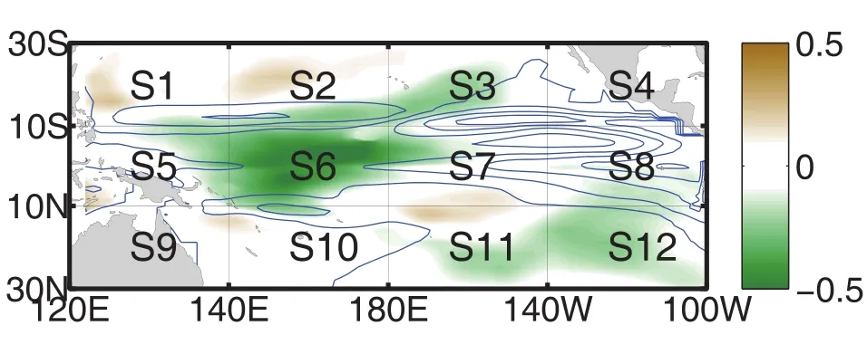
Fig.3.Horizontal distribution of the identi fied CNOPs for SST(shaded;units:°C)and SL(blue contours),and the distribution of the divided target areas for experiments(referred to as S1,S2···).Each area is a 40°(lon)×20°(lat)rectangle.

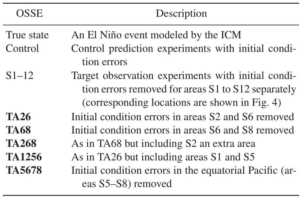
Table 1.Description of the control prediction experiments and target observation experiments based on the idealized OSSEs.The CNOP-related(multi-area)target observation experiments are marked in bold.

In short,the target observation experiments are designed in two parts: one to identify the most effective subregion(sensitive area)by observing various single target regions;and another to further investigate the effect of multi-area observation on ENSO prediction.The latter experiments can evaluate the effectiveness of removing initial condition errors in the CNOP-related areas on El Ni˜no prediction.

第二，利用机会，克服自身“短板”。要充分利用国家赋予的九大政策优势，引进国内外先进医疗机构、高端医疗人才和先进的医疗器械、前沿医疗技术，提升海南高端医疗服务的能力，为医疗旅游产业发展奠定基础。而私立医疗机构是高端医疗旅游产品供给的主力军，要出台相关政策吸引社会资本及海外资本投资医疗机构、医疗器械等相关领域。

3.Results from the control prediction experiments

In this section,we present in detail the results from the control prediction experiments.These results are used to measure the effectiveness of the target observations on ENSO predictions.

Note that the predicted El Ni˜no evolution can be deviated from the “true”ENSO event when errors in initial conditions of SST and SL components are superimposed.By subtracting SST anomalies in the “true”state from those in the control prediction experiments,the error evolutions induced by added initial SST and SL errors are calculated as follows:

in whichASST,true(i,j,t)is the “true”SST anomaly at monthtand ocean model grid(i,j);andASST,f(i,j,t)is the predicted SST anomaly with initial condition errors.Then,ESST(i,j,t)represents the initial-error-induced SST error growth for atmonth lead-time prediction.In terms of error growth,the SST error growth induced by the initial error is strongly seasonally dependent,which is known as the SPB phenomenon.To demonstrate the seasonal evolution of the error growth,the error growth rate in the Ni˜no3.4 area is defined as follows:

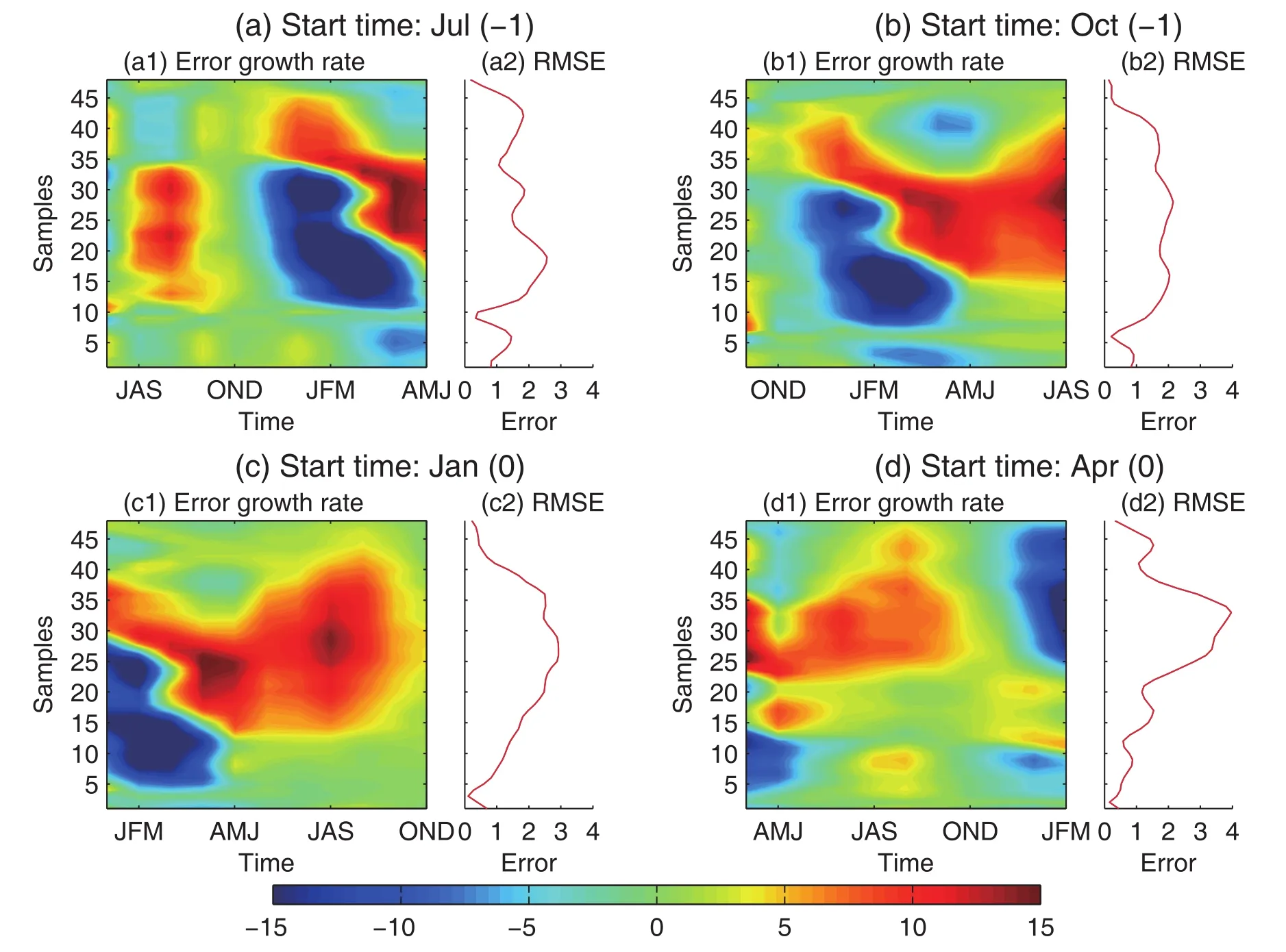
Fig.4.Error growth rate and RMSE(units:°C)of the SST in the Ni˜no3.4 area,which are obtained from different start months in the control prediction experiments:(a)July(−1);(b)October(−1);(c)January(0);(d)April(0).The vertical axes denote 48 samples of initial condition errors.

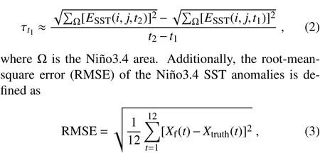
whereXf(t)andXtruth(t)denote the predicted and “truth”Ni˜no3.4 index at montht,respectively.

The error growth rate and RMSE of the Ni˜no3.4 SST anomaly are shown in Fig.4.Clearly,large error growth is generally accompanied by a strong SPB phenomenon.Regardless of the start time when making the prediction,the largest error growth rate often emerges during spring(April–May–June)and summer(July–August–September).The predicted error growth from summer is much more restrained than that from winter.For example,the RMSE tends to be lower than 2°C when predictions are made at the start month July(−1)(Fig.4a2),while the RMSE can attain its maximum(larger than 3°C)when performing a prediction at the initial month January(0)(Fig.4c2).In addition,large error growth(e.g.,RMSE greater than 1.5°C)is often accompanied by a prominent SPB phenomenon.It is once again indicated that the SPB is one of the major factors limiting the prediction skill.

4.Efficiency of the S1–12 target observations

This section explores the sensitive areas for target observation in El Ni˜no predictions.As demonstrated in section 2.2,the tropical Pacific is purposely divided into 12 subregions,and the initial condition errors in SST and SL in the S1–12 areas are removed(this can be achieved,for example,by adding extra observations in these areas for S1–12 target observations,respectively).In order to directly reveal the effectiveness,an efficiency index(EI)is defined as follows:

in which RMSEcf,stand RMSETA,stdenote the RMSE from the control prediction experiments and target observation experiments,respectively;the subscript TA represents the target area for observation(i.e.,S1,S2,...),and st is the start time when making the prediction.A positive value of EI signifies improvement in prediction skill,while a negative value means a worsened outcome.The larger the EI,the more effectively the ENSO prediction is improved when initial errors are reduced in the corresponding subregion.In other words,EI is an indicator of the sensitivity to which ENSO predictions can be affected through the initial conditions(i.e.,the closer EI is to 1,the more sensitive the area).

Figures 5 and 6 display a scatterplot of positive EI and the corresponding boxplot for the S1–12 target observation experiments,respectively.As clearly shown,removing the initial condition errors in the south subtropical Pacific(i.e.,areas S9–12)has no effect on the prediction accuracy of the El Nin˜o event(EI is close to 0).This implies that ENSO predictions are insensitive to the initial conditions in the south subtropical Pacific.However,eliminating the initial errors in the north of the central equatorial Pacific(i.e.,area S2)can enhance the forecast skill,which is indicated by reducing the errors by 15%.More sensitive areas are found along the equatorial Pacific,especially in the central(S6)and eastern(S8)Pacific,respectively.When removing initial error fields in area S6,for example,the prediction error tends to be reduced by 25%and even reaches 45%(Fig.6).In particular,the EI tends to drop quickly as the RMSE from the control prediction experiments increases.This reveals that the initial condition errors in other subregions,except for the current target area,may play a critical role in predictive error growth.Thus,to limit the error growth,multiple subregions should be considered simultaneously for target observations.

One more thing that should be noted here is that removing the initial errors in one target area may worsen the prediction(Yu et al.,2012).The probability distribution for the improved prediction skill from the S1–12 target observation experiments is shown in Fig.7.It is shown that removing the initial condition errors in the central equatorial Pacific(area S6)during July(−1)to June(0)is always able to improve the ENSO prediction skills.Strong uncertainty exists in the enhancement of the prediction skill by adding observations in other subregions(i.e.,S5 and S8).That is,deploying observations only in one subregion during certain seasons may fail to yield a better prediction result.Compared with the control prediction experiments,for example,observing in area S8 tends to yield a worse prediction when making predictions during autumn and winter,compared with the control prediction experiments(e.g.,the probability for improvement is less than40%).In this sense,it is evident that adding observations in the central Pacific is wise for improving the prediction skill using the ICM. Additionally, it is also revealed that a seasonvarying observation strategy can further improve the El Ni˜no prediction skill with the ICM.

5.CNOP-related observing strategy

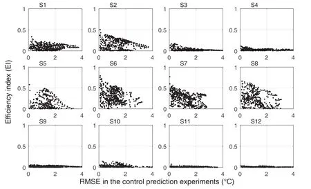
Fig.5.Scatterplots of the EI for the 12 target observation experiments based on the corresponding area described in Fig..3.Here,the x-coordinate denotes the RMSE of the Ni˜no3.4 index(referred to as E-Ni˜no3.4)from the control prediction experiments.The y-coordinate denotes the EI for target observations.Note that negative EI is not shown.

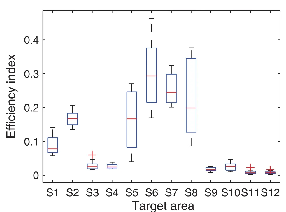
Fig.6.Boxplot of the ensemble mean EI for 12 start times in the S1–12 target observation experiments.The red strigula represents median efficiency among the El Ni˜no predictions in the onset year.The maximal and minimal efficiency,along with upper and lower quartile(blue bar),are also shown to indicate the uncertainties in improving ENSO prediction.Note that the negative efficiency indexes are excluded.

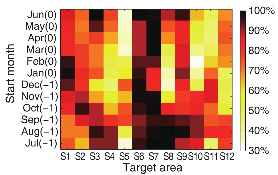
Fig.7.Probability distributions for improved prediction skill in the 12 target areas as a function of different start times.

Section 4 illustrates the effectiveness of target observations in different subregions on improving El Ni˜no predictions in the ICM.The S1–12 target observation experiments indicate that additional observations in the central and eastern Pacific can improve the prediction skill.In addition,initial condition errors in some areas(e.g.,area S2)are also crucial for inducing prediction error growth in some cases.As demonstrated in Tao et al.(2017),who identified CNOPs in the ICM,the ENSO prediction skill is quite sensitive to the initial states in the central and eastern Pacific.The results derived from the target observation experiments also certify the sensitive areas determined by the CNOP approach.Besides,Tao et al.(2017)also showed that the CNOPs derived from the ICM are strongly dependent on the seasons.For example,the CNOPs in winter reveal that the sensitive areas are located in the central and eastern equatorial Pacific(i.e.,the S6 and S8 subregions),and the CNOPs in summer reveal that the sensitive areas are located in the central equatorial tropical Pacific and its north(i.e.,the S2,and S6 subregions).Thus,CNOP-related target observation experiments(including TA26,TA68,TA268,TA1256 and TA5678)are implemented to explore the effectiveness of multi-subregion observations on improving prediction skill.

Table 2 shows the statistical mean of the RMSE and the relevant EI from the CNOP-related target observation experiments.The prediction errors are largely reduced(e.g.,the EI is larger than 0.4).Clearly,the TA5678 observational strategy,which is similar to the TAO array observational network,is optimal in terms of ENSO predictions.The mean prediction error(about 0.42°C)is much lower than that from the control prediction experiments(mean RMSE is 1.57°C).In contrast,although the TA1256 observational network(i.e.,the western and central Pacific)has an approximately equal size area as TA5678 for observations,the resultant prediction errors are larger.Figure 8 displays the monthly mean RMSE from the CNOP-related target observation and control prediction experiments.A strongly season-dependent prediction skill can be found based on the TA1256 observational network;the prediction errors are greatly reduced(e.g.,the prediction error is less than 0.7°C)when performing the prediction during winter,whereas the prediction errors tend to be larger than 1.1°C when the prediction time begins in summer.Such seasonality leads to a poor performance.It can be seen that the TAO array,at least based on those idealized experiments,is a relatively effective observation strategy.

However,considering the high cost for large-area observations and maintenance,it is practically impossible to widely deploy intensive observations,at least for the moment.Further experiments show that a relatively small-scale observational network can achieve a similar effect to the large-scale observational network.Strikingly,the TA26 target observation experiments,in which observations are carried out only in the central equatorial Pacific and the north(the S2 and S6 subregions),show a similar prediction effect to the TA1256 target observation experiments(e.g.,the mean RMSE is 0.92°C based on the TA26 observational network,and 0.9°C based on the TA1256 observational network).Thus,under the situation of the limited capacity,observations should be preferentially deployed in the central equatorial Pacific and its north instead of the TA1256 observational network.Certainly,observing in the eastern Pacific is equally important.Predictions based on the TA68 observational network,in which initial condition errors are reduced in the central and eastern equatorial Pacific,are as skillful as the TA26 observational network.Nevertheless,the prediction skill diあers among initial seasons. In the TA68 target observation experiments,the prediction skill is high at the initial timein summer but low in winter(Fig.8),which is contrary to the case for TA26.It is con firmed that the sensitive areas for El Ni˜no predictions are dependent on the initial season.Thus,a seasonally varying observational strategy is preferable to optimally improve the ENSO prediction skill.For example,on the basis of the TA26 observing strategy,adding observations in the eastern equatorial Pacific from April to October can effectively reduce the prediction error to be lower than 0.6°C(i.e.,EI=(1.57−0.6)/0.6≈0.62).Moreover,such seasondependent observation has advantages over a stationary observational strategy(e.g.,the prediction error is about 0.66°C based on the TA268 observational network).

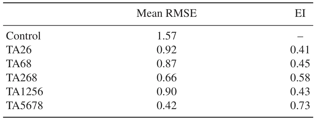
Table 2.Mean RMSE(units:°C)and EI from the CNOP-related target observations.

Fig.8.Monthly mean RMSE(units:°C)of Ni˜no3.4 index for various observing strategies as a function of the initial forecast month.The CPEs denotes control prediction experiments.

To further demonstrate the efficiency of the CNOP-related observational strategy on ENSO prediction skill,the error growth tendency is calculated[using Eq.(2)].The results from the TA26,TA68 and TA268 target observation experiments are shown in Figs.9–11,respectively.Clearly,the SPB phenomenon is markedly weakened such that the RMSEs are lower than those in the control prediction experiments.In addition,each observational network differs in terms of the weakening of the SPB phenomenon when making predictions from different initial seasons.For example,based on the TA26 observational network,the SPB phenomenon is remarkably weakened when performing predictions from winter and spring(Figs.9c and d),and thus the error growth is effectively reduced;whereas,a strong SPB phenomenon still emerges even though initial condition errors in the S2 and S6 subregions are removed in summer(Fig.9a).On the contrary,in the TA68 target observation experiments,the SPB phenomenon is weakened when predictions are made in summer(Fig.10a).It is indicated that it is preferential to deploy the TA68 observational network in summer and the TA26 observational network in winter.Compared with the TA26 target observation experiments,it is interesting to find that TA268 is not conducive to a weakened SPB phenomenon(as shown in Fig.11)when predictions are performed in winter.Clearly,the effects of an oceanic observing network on a reduction in the SPB phenomenon are seasonally dependent.This may be related to the fact that the onset,development and maturation of ENSO events are strongly seasonally dependent,with the maximum interannual SST anomalies occurring in winter and minimum ones in spring.Further investigations on these issues are clearly needed in the future.

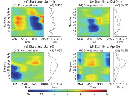
Fig.9.As in Fig.4 but for the TA26 target observation experiments.The red line is for the RMSE of Ni˜no3.4 index in the TA26 target observation experiments,and the blue line is for the control prediction experiments.

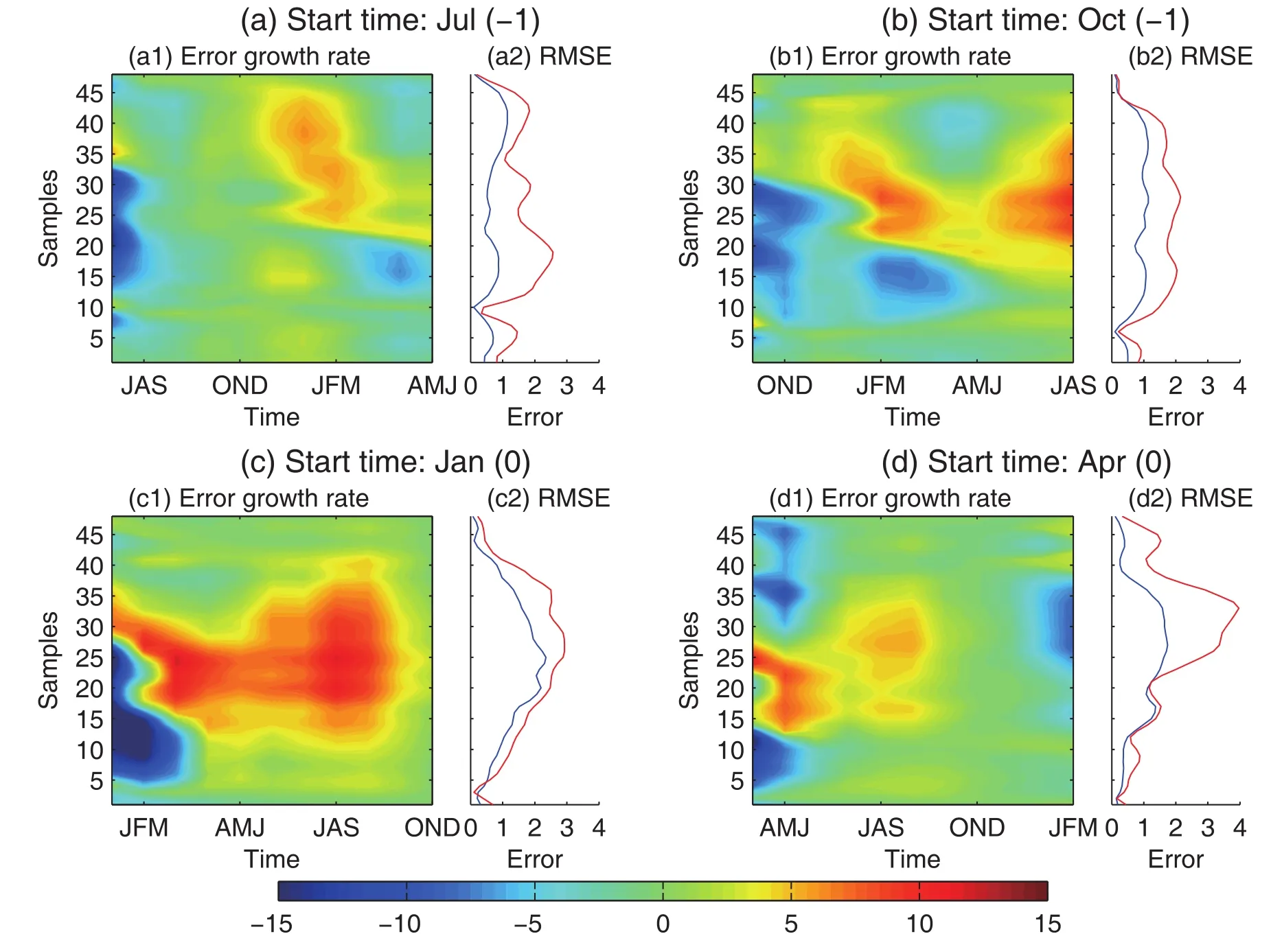
Fig.10.As in Fig.4 but for the TA68 target observation experiments.The red line is for the RMSE of Ni˜no3.4 index in the TA68 target observation experiments,and the blue line is for the control prediction experiments.

Note that improved initial conditions in sensitive areas can weaken the SPB phenomenon,thus enhancing the ENSO prediction skill.Although some observational strategies can reduce the prediction errors,the SPB phenomenon may not be suppressed and may even be strengthened.In addition,it is demonstrated that a season-varying observation strategy is quite effective for improving El Ni˜no predictions,and thus weakening the SPB phenomenon.

6.Conclusion

This study is an extension of Tao et al.(2017),in which the sensitive areas for ENSO predictions are identi fied using the CNOP approach and the ICM developed by Zhang et al.(2003).As suggested in Tao et al.(2017),a season-based target observation(in particular,deploying observations in the central and eastern equatorial Pacific)may greatly improve the ENSO prediction skill and profoundly weaken the SPB phenomenon.However,Tao et al.(2017)did not explore the extent to which CNOP-related target observations can improve the prediction skill of El Ni˜no events.

In this paper,OSSEs are performed to demonstrate the extent to which ENSO predictions can be improved by removing initial condition errors in some areas of focus(i.e.,sensitive areas)in the ICM.The idealized OSSEs include two groups of experiments using the ICM:control prediction experiments and target observation experiments.The former are implemented with initial condition errors constructed using an ensemble-based algorithm,while the latter serve as an idealized target observation system to investigate the effi-ciency with which the prediction skill can be improved.

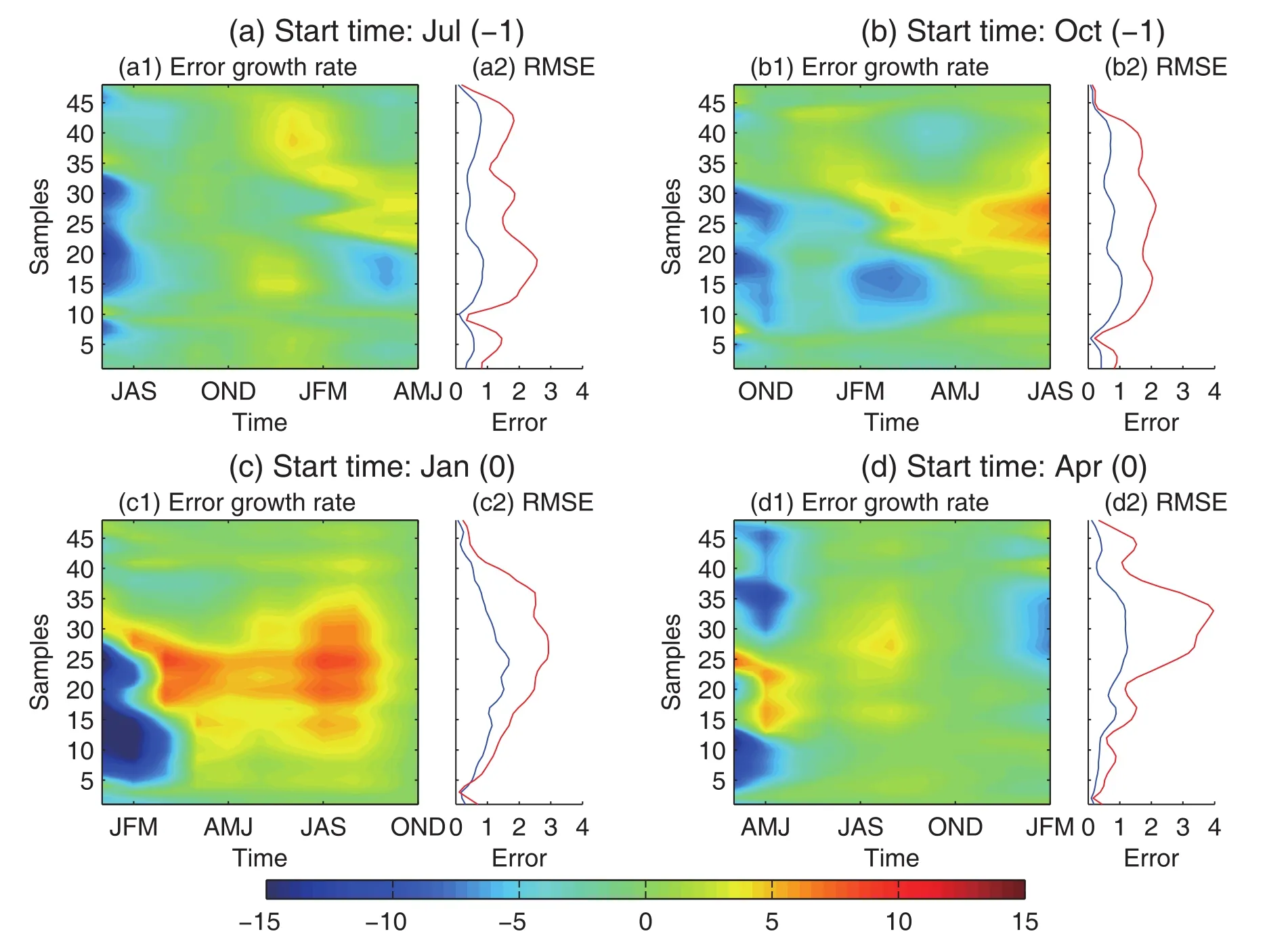
Fig.11.As in Fig.4 but for the TA268 target observation experiments.The red line is for the RMSE of Ni˜no3.4 index in the TA268 target observation experiments,and the blue line is for the control prediction experiments.

The control prediction experiments show that the prediction skill is strongly influenced by the SPB phenomenon in the ICM.Based on the target observation experiments for areas S1–S12,we investigate the importance of observing in these 12 different target areas of the tropical Pacific.The indication is that the El Ni˜no prediction skill is sensitive to the initial state in the central and eastern equatorial Pacific,which are also the CNOP-determined areas.Eliminating the initial errors in the central equatorial Pacific can successfully reduce the prediction errors by 25%.In addition,large uncertainty exists in the enhancement of prediction skill by adding observations in one subregion,except in subregion S6 and S7(i.e.,the central equatorial Pacific).All these results imply the significance of the initial state in the central Pacific for El Ni˜no prediction.Nevertheless,the initial errors in other areas cannot be ignored.Note that the prediction skill from the target observation experiments tends to decline quickly as the prediction errors become larger from the control prediction experiments.This reveals that initial condition errors in other areas play a critical role in prediction error growth.Thus,multi-subregion observations should be deployed simultaneously to limit the error growth.Further,the CNOP-related target observation experiments show considerable advantages in improving the ENSO prediction skill.Removing the initial condition errors in S2 and S6(i.e.,the central equatorial Pacific and its north)can improve the model prediction skill by 41%(i.e.,EI=0.41).Observation in the eastern Pacific is equally important.Based on the TA68 observational network,the prediction of ENSO is as skillful as based on the TA26 observational network.However,the prediction skill differs from one season to another.Thus,a time-varying observational network would be a reasonable approach to improving the prediction skill.For example,in addition to observing in the central equatorial Pacific and its north all year round,increasing observations(e.g.,ship-board ADCPs)in the eastern equatorial Pacific during April to October is crucially important,which can increase the forecast accuracy by 62%.Such a season-varying observing strategy can greatly reduce the SPB phenomenon and then limit the error growth induced by the initial condition errors.On the other hand,it is worth noting that additional observations in non-sensitive areas may not be beneficial in weakening the SPB,and may even strengthen this phenomenon.

From the target observation perspective,our study verifies the sensitive areas determined by the CNOP approach and further assesses the effects of CNOP-related target observations on El Ni˜no prediction skill.Particularly,deploying a time-varying observational network is strongly advised,to markedly improve El Ni˜no prediction.Note that a new international program aimed at building an internationally coordinated and sustainable tropical Pacific observing system(named TPOS)began in 2014 and is expected to be completed in 2020(Cravatte et al.,2015).The target observation experiments or the CNOP approach provide theoretical guidance for designing a reasonable and effective observational network in the tropical Pacific.

Note that in this study we simply remove the initial condition errors,instead of using assimilation techniques for prediction initialization.However,previous studies have in-dicated that ENSO prediction skill is highly dependent on the initialization scheme or assimilation approach,as well as the model itself(Rosati et al.,1997;Toth and Kalnay,1997;Chen et al.,1995;Zheng et al.,2006;Zhu et al.,2012).Thus,the resultant prediction skill may be overestimated in this work.Additionally,the model errors are ignored in the experiments.Thus,some questions should be addressed further in future work:What is the effect on prediction skill if an advanced data assimilation method is introduced into the ICM?When considering model errors,to what extent can target observations improve the ENSO prediction skill?It is worth mentioning that Gao et al.(2016)successfully implemented a 4DVar data assimilation method into the ICM.Such work offers technical support for future studies on ENSO prediction skill.Thus,in future work,we intend to carry out OSSEs to estimate the effect of sensitive areas when using 4DVar data assimilation.Furthermore,model errors will also be considered in these related modeling studies.

7.Discussion

It has been widely recognized in recent decades that initial condition errors in the central and eastern tropical Pacific can have significant effects on ENSO prediction.For example,Mu et al.(2014)stressed that observing in the central and eastern tropical Pacific(so-called sensitive areas)not only can reduce the initial errors,but also capture the signal of El Ni˜no in advance,so as to effectively improve the prediction of ENSO.However,as mentioned in the introduction,the sensitive areas identified for ENSO prediction may differ somewhat.Here,a more detailed discussion is given to address the uncertainty issues related to the sensitive areas identified from different studies.

According to the definition of target observation(Snyder,1996;Mu et al.,2009),to better predict an event at a future time t1(verification time)in an area of focus(verification area),additional observations should be deployed at a future time t2(target time,t2＜t1)in certain special areas(sensitive areas),where additional observations are expected to make a large contribution to reducing the prediction errors in the verification area.Consequently,the identified sensitive areas are logically dependent on the times,including the initial time and verification time,verification areas,the variables to be focused upon(i.e.,“precursors”),and the model itself.

7.1.Dependence on initial time and verification time

Using a hybrid coupled model,Fan et al.(2000)found that the role of the western and eastern tropical Pacific relies critically on the lead time of prediction:The initial signal in the western Pacific is most significant for the prediction of a three-month lead time,while the role of the eastern Pacific becomes dominant for predictions at longer leads.In Tao et al.(2017),it is clearly shown that the sensitive areas for ENSO prediction are significantly season-dependent.Some studies have also shown that the error growth induced by optimalinitial errors is seasonally dependent (i.e., an SPB-like errorevolution) and ENSO-phase-dependent(i.e.,a larger error growth occurs for El Ni˜no than La Ni˜na)(Moore and Kleeman,1997a,b;Yu et al.,2009).

7.2.Areas to be chosen for verification

Anomalies of SST in eastern tropical Pacific are important during the ENSO cycle;therefore,we usually recognize the Ni˜no3.4 area as the verification area for target observations.However,the prediction of the central Pacific is equally important,especially for the so-called central Pacific El Ni˜no.Tang et al.(2006)investigated the optimal initial SST anomaly patterns using different verification areas(e.g.,Ni˜no3,Ni˜no4,and the entire basin),suggesting that the sensitive areas can be different as the prediction area differs.For instance,to predict the SST in the Ni˜no3 area,the uncertainties in initial states in the eastern and central Pacific are most favored for the error growth.When using the Ni˜no4 area as the verification area,the function of the initial states in the western Pacific Ocean becomes prominent.

7.3.Variables to be observed

Identifying the most important precursors and corresponding sensitive areas is also important for target observations.However,differences exist among different models.Some studies have found that thermocline information is much more important than surface information for SST prediction(Moore and Kleeman,1996;Xue et al.,1997a,b).When using a different model,Fan et al.(2000)argued that the initial states of the SST and thermocline field are equally important for SST prediction.By contrast,Tang et al.(2006)considered that the uncertainties in SST are much more important than thermocline perturbations.Such contradictions may be attributable to the different representations of subsurface feedback in models.On the other hand,Wang et al.(2017)used ocean currents as a precursor,and suggested that the information on ocean currents near the dateline and the southern edge of the South Equatorial Current is crucial for El Ni˜no prediction.In their work,a statistical model based on the identified precursor(i.e.,ocean currents)was developed,with high ENSO prediction skill.

7.4.Models with various complexities

Lastly,the greatest challenge in identifying sensitive areas is the model itself.Because a predictive model is generally an approximation of the earth system,model errors that can be different from each other often exist,which has a large influence on the determination of sensitive areas in the real climate system.As an illustration,Moore and Kleeman(2001)investigated the differences between optimal perturbations using various versions of coupled models,concluding that the nonlinearities in models can have a significant impact on the structure of the optimal perturbations.That is,the identified sensitive areas are noticeably dependent on the model.As a result,the sensitive areas are also influenced by the complexity of models.By calculating the SV in an intermediate-complexity model introduced by Battisti(1988),Chen et al.(1997)implied that the predicted SST anomaly is sensitive to the initial state in the southeastern tropical Pacific.A similar result was also found in Thompson(1998).Besides,Fan et al.(2000),using a hybrid coupled model,stressed the importance of information in the Northern Hemisphere ITCZ.Moore et al.(2003)further compared different versions of a hybrid coupled model,and concluded that the sensitive areas are located in the central and eastern Pacific when using statistical models of the atmosphere,while they are mainly located in the warm pool when adding a parameterization for deep atmospheric convection into the coupled model.For a more complex model(e.g.,a CGCM such as GMAO CGCMv1),Tang et al.(2006),also considered that the initial SST information in the central and eastern Pacific is important to accurately predict the SST in the tropical Pacific;whereas,according to the studies of Duan and Wei(2013)and Duan and Hu(2016),the subsurface signal in the western and eastern Pacific is crucial for the prediction of El Ni˜no because this region can afterwards feed back to the surface via equatorial waves and thermodynamic effects.

Furthermore,a growing number of studies have focused on the contributions to ENSO prediction of processes in the extratropical Pacific and beyond the Pacific(Penland and Sardeshmukh,1995;Zhangetal.,1998;Newmanetal.,2011;Frauen and Dommenget,2012;Boschat et al.,2013;Keenlyside et al.,2013),and its interdecadal dependence(Penland and Matrosova,2006;Aiken et al.,2015).Keenlyside et al.(2013),for example,demonstrated the important role of the equatorial Atlantic in enhancing El Ni˜no prediction.Also,Aiken et al.(2015)showed that SST anomalies in the Indian and South Atlantic oceans become important as the prediction time increases.Hence,identifying the most sensitive area for ESNO prediction remains a huge challenge.Despite the above-stated factors limiting the way we can discern these sensitive areas,CNOP-based studies,like this one,can improve our understanding of ENSO predictability.

Acknowledgements.The authors thank Profs.Mu MU and Qiang WANG for their insightful comments and constructive suggestions.We also wish to thank the anonymous reviewers for the same.This research was supported by the Strategic Priority Research Program of the Chinese Academy of Sciences(Grant No.XDA19060102),the National Natural Science Foundation of China(Grant Nos.41475101,41690122,41690120 and 41421005),the National Programme on Global Change and Air–Sea Interaction Interaction(Grant Nos.GASI-IPOVAI-06 and GASI-IPOVAI-01-01),and the Taishan Scholarship.

REFERENCES

Aiken,C.M.,A.Santoso,S.McGregor,and M.H.England,2015:Optimal forcing of ENSO either side of the 1970’s climate shift and its implications for predictability.Climate Dyn.,45,47–65,https://doi.org/10.1007/s00382-014-2300-8.

Bishop,C.H.,B.J.Etherton,and S.J.Majumdar,2001:Adaptive sampling with the ensemble transform Kalman filter.Part I:Theoretical aspects.Mon.Wea.Rev.,129,420–436,https://doi.org/10.1175/1520-0493(2001)129＜0420:ASWTET＞2.0.CO;2.

Bishop,C.H.,and Z.Toth,1999:Ensemble Transformation and Adaptive Observations.J.Atmos.Sci.,56,1748–1765,https://doi.org/10.1175/1520-0469(1999)056＜1748:ETAAO＞2.0.CO;2.

Boschat G.,P.Terray,and S.Masson,2013:Extratropical forcing ofENSO.Geophys.Res.Lett.,40,1605–1611.https://doi.org/10.1002/grl.50229.

Chen,D.K.,and M.A.Cane,2008:El Ni˜no prediction and predictability.J.Comput.Phys.,227,3625–3640,https://doi.org/10.1016/j.jcp.2007.05.014.

Chen,D.K.,S.E.Zebiak,A.J.Busalacchi,and M.A.Cane,1995:An improved procedure for EI Nino forecasting:Implications for predictability.Science,269,1699–1702,https://doi.org/10.1126/science.269.5231.1699.

Chen,Y.-Q.,D.S.Battisti,T.N.Palmer,J.Barsugli,and E.S.Sarachik,1997:A study of the predictability of tropical Pacific SST in a coupled atmosphere–ocean model using singularvector analysis: The role of the annual cycle and the ENSO cycle.Mon.Wea.Rev.,125,831–845.

Cravatte,S.,A.Ganachaud,B.Dewitte,and F.Hernandez,2015:TPOS2020:Tropical Pacific observing system for 2020.Mercator Ocean-Coriolis Quarterly Newsletter,27–33.

Duan,W.S.,and C.Wei,2013:The ‘spring predictability barrier’for ENSO predictions and its possible mechanism:Results from a fully coupled model.Int.J.Climatol.,33(5),1280–1292,https://doi.org/10.1002/joc.3513.

Duan,W.S.,and J.Y.Hu,2016:The initial errors that induce a signi ficant“spring predictability barrier”for El Ni˜no events and their implications for target observation:results from an earth system model.Climate Dyn.,46,3599–3615,https://doi.org/10.1007/s00382-015-2789-5.

Duan,W.S.,X.C.Liu,K.Y.Zhu,and M.Mu,2009:Exploring the initial errors that cause a signi ficant“spring predictability barrier”for El Ni˜no events.J.Geophys.Res.,114,https://doi.org/10.1029/2008JC004925.

Fan,Y.,M.R.Allen,D.L.T.Anderson,and M.A.Balmaseda,2000:How predictability depends on the nature of uncertainty in initial conditions in a coupled model of ENSO.J.Climate,13,3298–3313,https://doi.org/10.1175/1520-0442(2000)013＜3298:HPDOTN＞2.0.CO;2.

Feder,T.,2000:Argo begins systematic global probing of the upper oceans.Physics Today,53,50–51,https://doi.org/10.1063/1.1292477.

Fl¨ugel,M.,and P.Chang,1998:Does the predictability of ENSO depend on the seasonal cycle?J.Atmos.Sci.,55,3230–3243,https://doi.org/10.1175/1520-0469(1998)055＜3230:DTPOED＞2.0.CO;2.

Frauen,C.,and D.Dommenget,2012:Influences of the tropical Indian and Atlantic Oceans on the predictability of ENSO.Geophys.Res.Lett.,39,L02706,https://doi.org/10.1029/2011GL050520.

Gao,C.,and R.H.Zhang,2017:The roles of atmospheric wind and entrained water temperature(Te)in the second-year cooling of the 2010-12 La Ni˜na event.Climate Dyn.,48,597–617,https://doi.org/10.1007/s00382-016-3097-4.

Gao,C.,X.R.Wu,and R.H.Zhang,2016:Testing a fourdimensional variational data assimilation method using an improved intermediate coupled model for ENSO analysis and prediction.Adv.Atmos.Sci.,33,875–888,https://doi.org/10.1007/s00376-016-5249-1.

Gao,C.,R.-H.Zhang,X.R.Wu,and J.C.Sun,2017:Idealized experiments for optimizing model parameters using a 4D-Variational method in an intermediate coupled model of ENSO.Adv.Atmos.Sci.,https://doi.org/10.1007/s00376-017-7109-z.(in Press)

Hu,J.Y.,and W.S.Duan,2016:Relationship between optimal precursory disturbances and optimally growing initial errors associated with ENSO events:Implications to target observationsforENSOprediction.J.Geophys.Res.,121,2901–2917,https://doi.org/10.1002/2015JC011386.

Keenlyside,N.,and R.Kleeman,2002:Annual cycle of equatorial zonal currents in the Pacific.J.Geophys.Res.,107,8-1–8-13,https://doi.org/10.1029/2000JC000711.

Keenlyside,N.S.,H.Ding,and M.Latif,2013:Potential of equatorial Atlantic variability to enhance El Nin˜o prediction.Geophys.Res.Lett.,40,2278–2283,0.1002/grl.50362.

King,J.C.,1997:Currents of change:El Nin˜o’s impact on climate and society.Weather,52,159–160,https://doi.org/10.1002/j.1477-8696.1997.tb06299.x.

Kumar,A.,H.Wang,Y.Xue,and W.Q.Wang,2014:How much of monthly subsurface temperature variability in the equatorial Pacific can be recovered by the speci fication of sea surface temperatures?J.Climate,27,1559–1577,https://doi.org/10.1175/JCLI-D-13-00258.1.

Latif,M.,A.Sterl,E.Maier-Reimer,and M.M.Junge,1993a:Climate variability in a coupled GCM.Part I:The tropical Pacific.J.Climate,6,5–21,https://doi.org/10.1175/1520-0442(1993)006＜0005:CVIACG＞2.0.CO;2.

Latif,M.,A.Sterl,E.Maier-Reimer,and M.M.Junge,1993b:Structure and predictability of the El-Nin˜o/southern oscillation phenomenon in a coupled ocean-atmosphere general circulation model.J.Climate,6,700–708,https://doi.org/10.1175/1520-0442(1993)006＜0700:SAPOTE＞2.0.CO;2.

Lee,P.,and Coauthors,2016:Observing system simulation experiments(OSSEs)using a regional air quality application for evaluation.Air Pollution Modeling and its Application XXIV,D.G.Steyn and N.Chaumerliac,Eds.,Springer,599–605,https://doi.org/10.1007/978-3-319-24478-597.

Lord,S.J.,E.Kalnay,R.Daley,G.D.Emmitt,and R.Atlas,1997:Using OSSEs in the design of the future generation of integrated observing systems.Proc.1st Symposium on Integrated Observing Systems,American Meteorological Society,Long Beach,CA.

Masutani,M.,and Coauthors,2010:Observing system simulation experimentsData Assimilation,W.Lahoz,B.Khattatov,and R.Menard,Eds.,Springer,647–679,https://doi.org/10.1007/978-3-540-74703-124.

McCreary,J.P.,1981:A linear stratified ocean model of the equatorial undercurrent.Philos.Trans.Roy.Soc.London,298,603–635,https://doi.org/10.1098/rsta.1981.0002.

McPhaden,M.J.,and Coauthors,1998:The tropical oceanglobal atmosphere observing system:A decade of progress.J.Geophys.Res.,103,14 169–14 240,https://doi.org/10.1029/97JC02906.

McPhaden,M.J.,S.E.Zebiak,and M.H.Glantz,2006:ENSO as an integrating concept in Earth science.Science,314,1740–1745,https://doi.org/10.1126/science.1132588.

Moore,A.M.,and R.Kleeman,1996:The dynamics of error growth and predictability in a coupled model of ENSO.Quart.J.Roy.Meteor.Soc.,122,1405–1446.

Moore,A.M.,and R.Kleeman,1997a:The singular vectors of a coupled ocean-atmosphere model of ENSO,Part I:Thermodynamics,energetics and error growth.Quart.J.Roy.Meteor.Soc.,123,953–981.

Moore,A.M.,and R.Kleeman,1997b:The singular vectors of a coupled ocean-atmosphere model of ENSO,Part II:Sensitivity studies and dynamical interpretation.Quart.J.Roy.Meteor.Soc.,123,983–1006.

Moore,A.M.,and R.Kleeman,2001:The differences between the optimal perturbations of coupled models of ENSO.J.Climate,14,138–163.

Moore,A.M.J.Vialard,A.Weaver,D.L.T.Anderson,R.Kleeman,and J.R.Johnson,2003:The role of air–sea interaction in controlling the optimal perturbations of low-frequency tropical coupled ocean–atmosphere modes.J.Climate,16,951–968.

Morss,R.E.,and D.S.Battisti,2004a:Designing effi-cient observing networks for ENSO prediction.J.Climate,17,3074–3089,https://doi.org/10.1175/1520-0442(2004)017＜3074:DEONFE＞2.0.CO;2.

Morss,R.E.,and D.S.Battisti,2004b:Evaluating observing requirements for ENSO prediction:Experiments with an intermediate coupled model.J.Climate,17,3057–3073,https://doi.org/10.1175/1520-0442(2004)017＜3057:EORFEP＞2.0.CO;2.

Mu,M.,W.S.Duan,and B.Wang,2003:Conditional nonlinear optimal perturbation and its applications.Nonlinear Processes in Geophysics,10,493–501,https://doi.org/10.5194/npg-10-493-2003.

Mu,M.,W.S.Duan,and B.Wang,2007a:Season-dependent dynamics of nonlinear optimal error growth and El Ni˜no-Southern Oscillation predictability in a theoretical model.J.Geophys.Res.,112,https://doi.org/10.1029/2005JD006981.

Mu,M.,H.Xu,and W.S.Duan,2007b:A kind of initial errors related to“spring predictability barrier”for El Ni˜no events in Zebiak-Cane model.Geophys.Res.Lett.,34,https://doi.org/10.1029/2006GL027412.

Mu,M.,F.F.Zhou,and H.L.Wang,2009:A method for identifying the sensitive areas in targeted observations for tropical cyclone prediction:Conditional nonlinear optimal perturbation.Mon.Wea.Rev.,137,1623–1639,https://doi.org/10.1175/2008MWR2640.1.

Mu,M.,Y.S.Yu,H.Xu,and T.T.Gong,2014:Similarities between optimal precursors for ENSO events and optimally growing initial errors in El Ni˜no predictions.Theor.Appl.Climatol.,115,461–469,https://doi.org/10.1007/s00704-013-0909-x.

Mu,M.,W.S.Duan,D.K.Chen,and W.D.Yu,2015:Target observations for improving initialization of high-impact oceanatmospheric environmental events forecasting.National Science Review,2,226–236,https://doi.org/10.1093/nsr/nwv021.

Newman,M.,M.A.Alexander,and J.D.Scott,2011:An empirical model of tropical ocean dynamics.Climate Dyn.,37,1823–1841,https://doi.org/10.1007/s00382-011-1034-0.

Palmer,T.N.,R.Gelaro,J.Barkmeijer,and R.Buizza,1998:Singular vectors,metrics,and adaptive observations.J.Atmos.Sci.,55,633–653,https://doi.org/10.1175/1520-0469(1998)055＜0633:SVMAAO＞2.0.CO;2.

Penland,C.,and L.Matrosova,1994:A balance condition for stochastic numerical models with application to the El Ni˜no-Southern Oscillation.J.Climate,7,1352–1372,https://doi.org/10.1175/1520-0442(1994)007＜1352:ABCFSN＞2.0.CO;2.

Penland,C.,and P.D.Sardeshmukh,1995:The optimal growth of tropical sea surface temperature anomalies.J.Climate,8,1999–2024,https://doi.org/10.1175/1520-0442(1995)008＜1999:TOGOTS＞2.0.CO;2.

Penland,C.,and L.Matrosova,2006:Studies of El Ni˜no and interdecadal variability in tropical sea surface temperatures using a nonnormal filter.J.Climate,19,5796–5815,https://doi.org/10.1175/JCLI3951.1.

Philander,S.G.H.,1983:El-Ni˜no southern oscillation phenomena.Nature,302,295–301,https://doi.org/10.1038/302295a0.

Rosati,A.,K.Miyakoda,and R.Gudgel,1997:The impact of ocean initial conditions on ENSO forecasting with a coupled model.Mon.Wea.Rev.,125,754–772,https://doi.org/10.1175/1520-0493(1997)125＜0754:TIOOIC＞2.0.CO;2.

Snyder,C.,1996:Summary of an informal workshop on adaptive observations and FASTEX.Bull.Amer.Meteorol.Soc.,77,953–961.

Tang,Y.,2002:Hybrid coupled models of the tropical Pacific:I Interannual variability.Climate Dyn.,19,331–342,https://doi.org/10.1007/s00382-002-0230-3.

Tang,Y.,and W.Hsieh,2002:Hybrid coupled models of the tropical Pacific-II ENSO prediction.Climate Dyn.,19,343–353,https://doi.org/10.1007/s00382-002-0231-2.

Tang,Y.,R.Kleeman,and S.Miller,2006:ENSO predictability of a fully coupled GCM model using singular vector analysis.Journal of Climate,19(14),3361–3377.

Tao,L.J.,R.H.Zhang,and C.Gao,2017:Initial error-induced optimal perturbations in ENSO predictions,as derived from an intermediate coupled model.Adv.Atmos.Sci.,34(6),791–803,https://doi.org/10.1007/s00376-017-6266-4.

Thompson,C.J.,1998:Initial conditions for optimal growth in a coupled ocean–atmosphere model of ENSO.J.Atmos.Sci.,55,537–557.

Toth,Z.,and E.Kalnay,1997:Ensemble forecasting at NCEP and the breeding method.Mon.Wea.Rev.,125,3297–3319,https://doi.org/10.1175/1520-0493(1997)125＜3297:EFANAT＞2.0.CO;2.

Wang,B.,and Z.Fang,1996:Chaotic oscillations of tropical climate:A dynamic system theory for ENSO.J.Atmos.Sci.,53,2786–2802,https://doi.org/10.1175/1520-0469(1996)053＜2786:COOTCA＞2.0.CO;2.

Wang,J.,Y.Lu,F.Wang,and R.H.Zhang,2017:Surface current in “hotspot”serves as a new and effective precursor for El Ni˜no prediction.Scientific Reports,7(1),166.

Webster,P.J.,1995:The annual cycle and the predictability of the tropical coupled ocean-atmosphere system.Meteor.Atmos.Phys.,56,33–55,https://doi.org/10.1007/BF01022520.

Wu,C.C.,J.H.Chen,P.H.Lin,and K.H.Chou,2007:Target edobservations of tropical cyclonemovement based on the adjoint-derived sensitivity steering vector.J.Atmos.Sci.,64,2611–2626,https://doi.org/10.1175/JAS3974.1.

Xue,Y.,M.A.Cane,and S.E.Zebiak,1997a:Predictability of a coupled model of ENSO using singular vector analysis.Part I:Optimal growth in seasonal background and ENSO cycle.Mon.Wea.Rev.,125,2043–2056.

Xue,Y.,M.A.Cane,S.E.Zebiak,and T.N.Palmer,1997b:Predictability of a coupled model of ENSO using singular vector analysis.PartII:Optimal growth and forecast skill.Mon.Wea.Rev.,125,2057–2073.

Yu,Y.S.,W.S.Duan,H.Xu,and M.Mu,2009:Dynamics of nonlinear error growth and season-dependent predictability of El Ni˜no events in the Zebiak-Cane model.Quart.J.Roy.Meteor.Soc.,135,2146–2160,https://doi.org/10.1002/qj.526.

Yu,Y.S.,M.Mu,W.S.Duan,and T.T.Gong,2012:Contribution of the location and spatial pattern of initial error to uncertainties in El Ni˜no predictions.J.Geophys.Res.,117,https://doi.org/10.1029/2011JC007758.

Zebiak,S.E.,and M.A.Cane,1987:A model el Ni˜no-southern oscillation.Mon.Wea.Rev.,115,2262–2278,https://doi.org/10.1175/1520-0493(1987)115＜2262:AMENO＞2.0.CO;2.

Zhang,J.,W.S.Duan,and X.F.Zhi,2015:Using CMIP5 model outputs to investigate the initial errors that cause the“spring predictability barrier”for El Ni˜no events.Science China Earth Sciences,58,685–696,https://doi.org/10.1007/s11430-014-4994-1.

Zhang,R.H.,L.M.Rothste in,and A.J.Busalacchi,1998:Origin of upper-ocean warming and El Ni˜no change on decadal scales in the tropical Pacific Ocean.Nature,391(6670),879–883,https://doi.org/10.1038/36081.

Zhang,R.H.,A.J.Busalacchi,and D.G.De Witt,2008:The roles of atmospheric stochastic forcing(SF)and oceanic entrainment temperature(Te)in decadal modulation of ENSO.J.Climate,21,674–704,https://doi.org/10.1175/2007JCLI1665.1.

Zhang,R.H.,S.E.Zebiak,R.Kleeman,and N.Keenlyside,2003:Ane winter mediate coupled model for ElNi˜nos imulation and prediction.Geophys.Res.Lett.,30,https://doi.org/10.1029/2003GL018010.

Zhang,R.H.,S.E.Zebiak,R.Kleeman,and N.Keenlyside,2005b:Retrospective El Ni˜no forecasts using an improved intermediate coupled model.Mon.Wea.Rev.,133,2777–2802,https://doi.org/10.1175/MWR3000.1.

Zhang,R.H.,F.Zheng,J.Zhu,and Z.G.Wang,2013:A successful real-time forecast of the 2010-11 La Ni˜na event.Scienti fic Reports,3,1108,https://doi.org/10.1038/srep01108.

Zhang,R.H.,A.J.Busalacchi,R.G.Murtugudde,E.C.Hackert,and J.Ballabrera-Poy,2004:A new approach to improved SST anomaly simulations using altimeter data:Parameterizing entrainment temperature from sea level.Geophys.Res.Lett.,31,https://doi.org/10.1029/2003GL019237.

Zhang,R.H.,R.Kleeman,S.E.Zebiak,N.Keenlyside,and S.Raynaud,2005a:An empirical parameterization of subsurface entrainment temperature for improved SST anomaly simulations in an intermediate ocean model.J.Climate,18,350–371,https://doi.org/10.1175/JCLI-3271.1.

Zheng,F.,J.Zhu,R.H.Zhang,and G.Q.Zhou,2006:Improved ENSO forecasts by assimilating sea surface temperature observations into an intermediate coupled model.Adv.Atmos.Sci.,23,615–624,https://doi.org/10.1007/s00376-006-0615-z.

Zhu,H.Y.,and A.Thorpe,2006:Predictability of extratropical cyclones:The in fluence of initial condition and model uncertainties.J.Atmos.Sci.,63,1483–1497,https://doi.org/10.1175/JAS3688.1.

Zhu,J.S.,B.H.Huang,L.Marx,J.L.KinterIII,M.A.Balmaseda,R.H.Zhang,and Z.Z.Hu,2012:Ensemble ENSO hindcasts initialized from multiple ocean analyses.Geophys.Res.Lett.,39,L09602,https://doi.org/10.1029/2012GL051503.