New analytic solutions of the space-time fractional Broer-Kaup and approximate long water wave equations
2018-03-14erdikYaslan
H. Çerdik Yaslan
Department of Mathematics, Pamukkale University, Denizli 20070, Turkey
Abstract In the present paper, the exp (-φ(ξ)) expansion method is applied to the fractional Broer-Kaup and approximate long water wave equations. The explicit approximate traveling wave solutions are obtained by using this method. Here, fractional derivatives are defined in the conformable sense. The obtained traveling wave solutions are expressed by the hyperbolic, trigonometric, exponential and rational functions.Simulations of the obtained solutions are given at the end of the paper.
Keywords: The fractional Broer-Kaup equations; The fractional approximate long water wave equations; Conformable derivative; exp (-φ(ξ)) expansion method; Traveling wave solutions.
1.Introduction
Nonlinear partial differential equations are important tools used to modeled nonlinear dynamical phenomena in different fields such as mathematical biology, plasma physics, solid state physics, and fluid dynamics [1] . The traveling wave solutions of nonlinear partial differential equations play an important role in the study of nonlinear physical phenomena such as fluid dynamics, water wave mechanics, meteorology,electromagnetic theory, plasma physics and nonlinear optics etc. In the recent decade, many methods have been developed for finding the traveling wave solutions such as the Jacobi elliptic function method [2] , the ansatz method [3] , the exp-( φ( η))) method [4] , exp-function method [5] , consistent Riccati expansion method [6] , the (G′/G)-expansion method[7] .
Waves have a major influence on the marine environment and ultimately on the planet climate. One of the most important and application classifications of marine waves is the shallow water wave. The shallow water equations describe the motion of water bodies wherein the depth is short relative to the scale of the waves propagating on that body and are derived from the depth-averaged Navier-Stokes equations[8] . These equations are used to describe flow in vertically well-mixed water bodies where the horizontal length scales are much greater than the fluid depth (i.e., long wavelength phenomena) and to model the hydrodynamics of lakes, estuaries, tidal flats and coastal regions, as well as deep ocean tides.The equations also, are used to study many physical phenomena such forces acting on off-shore structures and in modeling the transport of chemical species such as storm surges, tidal fluctuations and tsunami waves [9] .
In the present paper, we consider space-time fractional approximate long water wave equations and Broer-Kaup equations which are used to model the bidirectional propagation of long waves in shallow water. The space-time fractional approximate long water wave equations (see, for example,[10-12] ) are given in the form
and the space-time fractional Broer-Kaup equations (see, for example, [13] ) are given as follows
Hereanddenote conformable fractional derivative with respect totandx, respectively. These equations have been investigated in [14-17] . New exact solutions for fractional DR equation and fractional approximate long water wave equation with the modified Riemann-Liouville derivative have been obtained by usingG′/G-expansion method in [14] . The time fractional coupled Boussinesq-Burger and time fractional approximate long water wave equations with conformable derivative by using the generalized Kudryashov method have been solved in [15] . The analytical approximate traveling wave solutions of time fractional Whitham-Broer-Kaup equations, time fractional coupled modified Boussinesq and time fractional approximate long wave equations have been obtained by using the coupled fractional reduced differential transform method in [16] . Here fractional derivative is defined by the Caputo sense. The fractional sub-equation method has been applied to the fractional variant Boussinesq equation and fractional approximate long water wave equation with Jumarie's modified Riemann-Liouville derivatives in [17] .
2.Description of the conformable fractional derivative and its properties
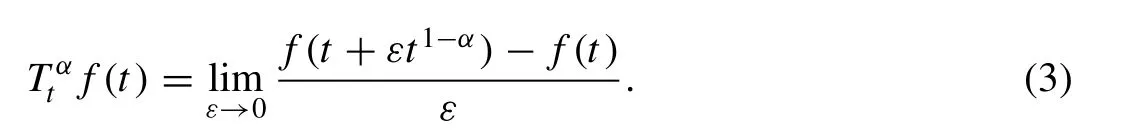
For a functionf: (0, ∞ ) →R, the conformable fractional derivative offof order 0 < α < 1 is defined as (see, for example, [18] )
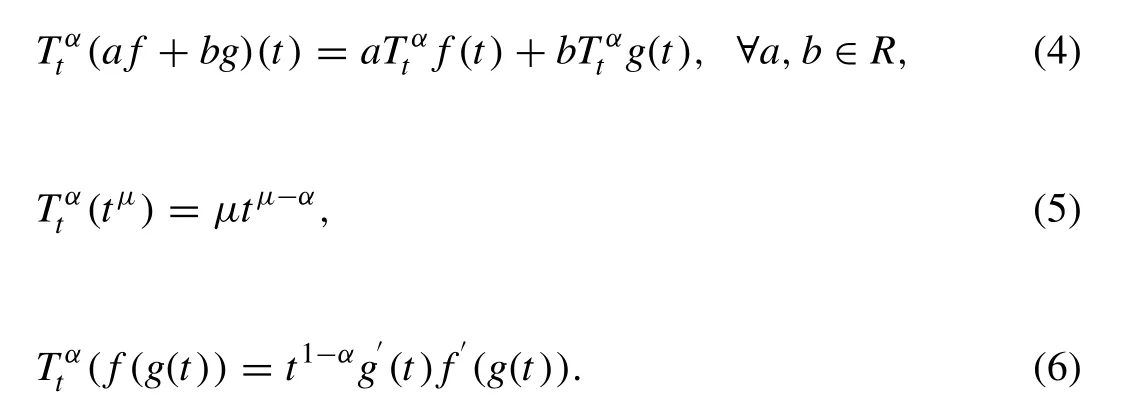
Some important properties of the conformable fractional derivative are as follows:
3.Analytic solutions to the space-time fractional approximate long water wave equations
Let us consider the following transformation

wherea,bare constants. Substituting (7) into (1) we have the following ordinary differential equations


Integrating (8) with respect to ξ, then we have
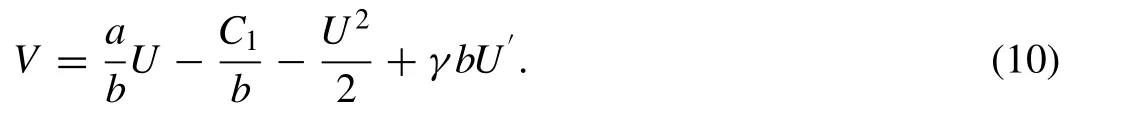
Substituting (10) into (9) yields
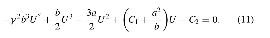
Here,C1andC2are integration constants. Let us suppose that the solution of (11) can be expressed in the following form:
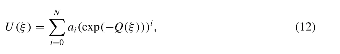
whereaiare constants to be determined later andQ( ξ) satisfies the following auxiliary ordinary differential equation:

Inserting (12) into (11) then by balancing the highest order derivative term and nonlinear term in result equation, the value ofNcan be determined as 1. Collecting all the terms with the same power of exp (-φ(ξ)) , we can obtain a set of algebraic equations for the unknownsa0,a1,C1,C2,a,b:

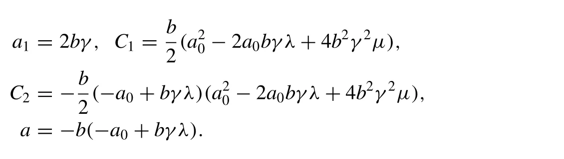
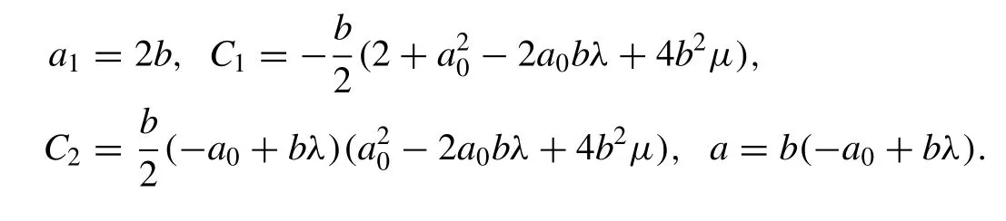
Solving the algebraic equations in the Mathematica, we obtain the following set of solutions:
The solutions of Eq. (1) are given as follows:

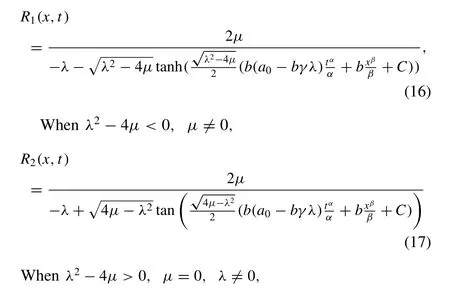
HereRi(x,t) ,i= 1 , 2, 3 , 4, 5 , is defined as follows:
When λ2-4µ > 0, µ / = 0,

Fig. 1. 3D plot of the solitary wave solution u 1 ( x, t ) of Eq. (1) for a 0 = 10, b = 1 , µ = 1 , C = 10, λ = 3 , γ = 10, α = 0. 75 , β = 0. 5 .


Here C is the integration constant.
Figs. 1-4 represent the change of amplitude and nature of the solitary waves for each obtained solitary wave solutions. The solutionsu1(x,t),u2(x,t) andv1(x,t)of Eq. (1) are simulated as traveling wave solutions for various values of the physical parameters in Figs. 1 -4 .Figs. 1 and 2 show solitary wave solutions of Eq. (1) . 3D plots of the obtained solutionsu1(x,t) andv1(x,t) are given in Fig. 1 and Fig. 2 for parametersa0= 10,b= 1 , µ=1 ,C= 10, λ = 3 , γ= 10, α = 0. 75 , β = 0. 5 , respectively.Figs. 3 and 4 are kink-type periodic wave solutions of Eq.(1) . 3D plot of the obtained solutionu2(x,t) is given for parametersa0= 0. 5 ,b= 1 , µ = 1 ,C= 5 , λ = 1 , γ = 1 α =0. 75 , β= 0. 5 in Fig.3 . Fig.4 demonstrates the same solution with 2D plot for 0 ≤x≤ 50 att= 1 .
4.Analytic solutions to the space-time fractional Broer-Kaup equations
Applying the transformation (7) into (2) we have the following ordinary differential equations

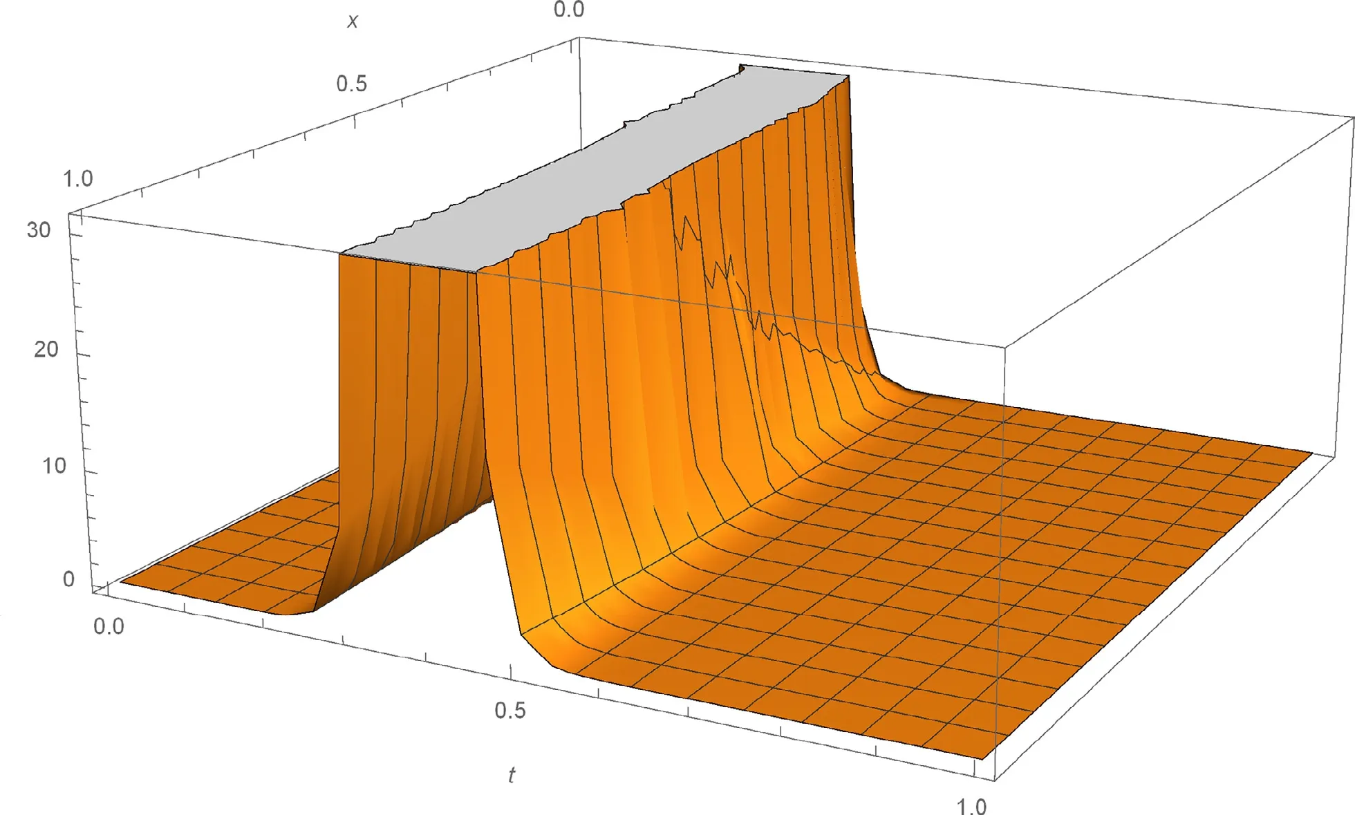
Fig. 2. 3D plot of the solitary wave solution v 1 ( x, t ) of Eq. (1) for a 0 = 10, b = 1 , µ = 1 , C = 10, λ = 3 , γ = 10, α = 0. 75 , β = 0. 5 .

Fig. 3. 3D plot of the periodic wave solution u 2 ( x, t ) of Eq. (1) for a 0 = 0. 5 , b = 1 , µ = 1 , C = 5 , λ = 1 , γ= 1 , α = 0. 75 , β = 0. 5 .
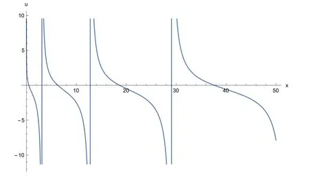
Fig. 4. 2D plot of the periodic wave solution u 2 ( x , 1) of Eq. (1) for a 0 = 0. 5 , b = 1 , µ = 1 , C = 5 , λ = 1 , γ = 1 , α = 0. 75 , β = 0. 5 .
Integrating (20) with respect to ξ, then we have
Substituting (22) into (21) yields

HereC1andC2are integration constants. Let us suppose that the solution of (23) can be expressed in the form (12) . Inserting (12) into (23) and balancing the highest order derivative term and nonlinear term in result equation, the value ofNcan be determined as 1. Collecting all the terms with the same power of exp (-φ(ξ)) , we can obtain a set of algebraic equations for the unknownsa0,a1,C2,C2,a,b:

Solving the algebraic equations in the Mathematica, we obtain the following set of solutions:

The solutions of Eq. (1) are given as follows:


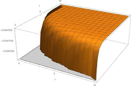
Fig. 5. 3D plot of the solitary wave solution u 1 ( x, t ) of Eq. (2) for a 0 = 0. 5 , b = 0. 7 , µ = 1 , C = 1 , λ = 3 , α = 0. 75 , β = 0. 5 .
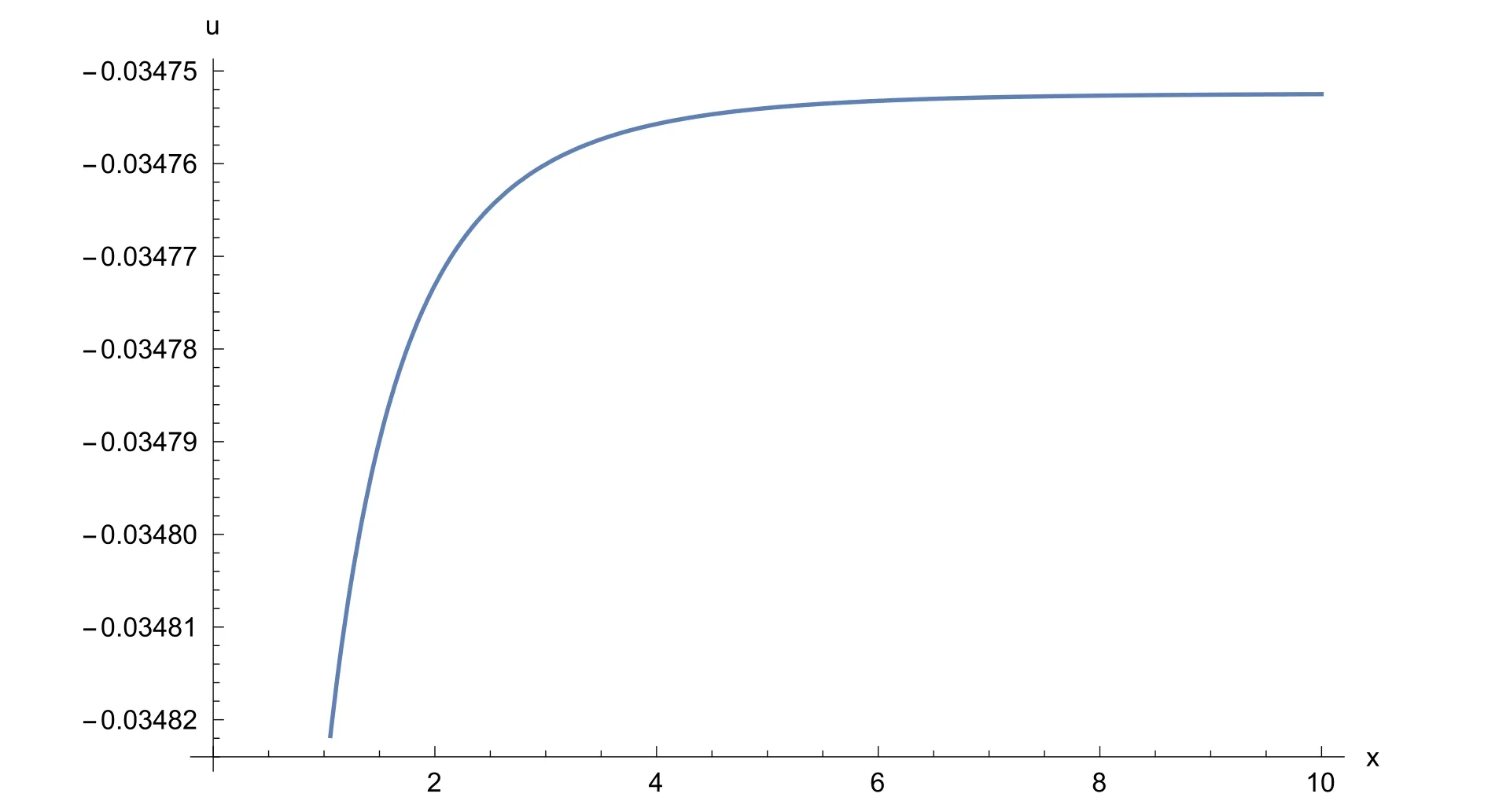
Fig. 6. 2D plot of the solitary wave solution u 1 ( x , 1) of Eq. (2) for a 0 = 0. 5 , b = 0. 7 , µ = 1 , C = 1 , λ= 3 , α = 0. 75 , β = 0. 5 .
When λ2-4µ = 0, µ = 0, λ = 0,
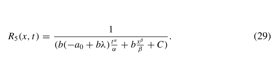

Fig. 7. 3D plot of the periodic wave solution v 2 ( x, t ) of Eq. (2) for a 0 = 0. 5 , b = 0. 7 , µ= 2, C = 1 , λ = 1 , α = 0. 75 , β = 0. 5 .
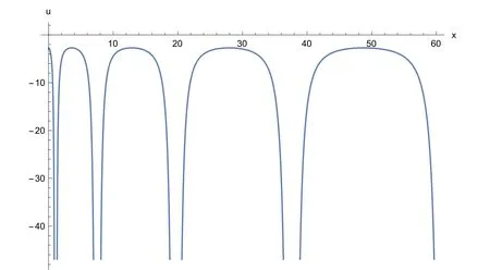
Fig. 8. 2D plot of the periodic wave solution v 2 ( x , 1) of Eq. (2) for a 0 = 0. 5 , b = 0. 7 , µ= 2, C = 1 , λ= 1 , α = 0. 75 , β = 0. 5 .
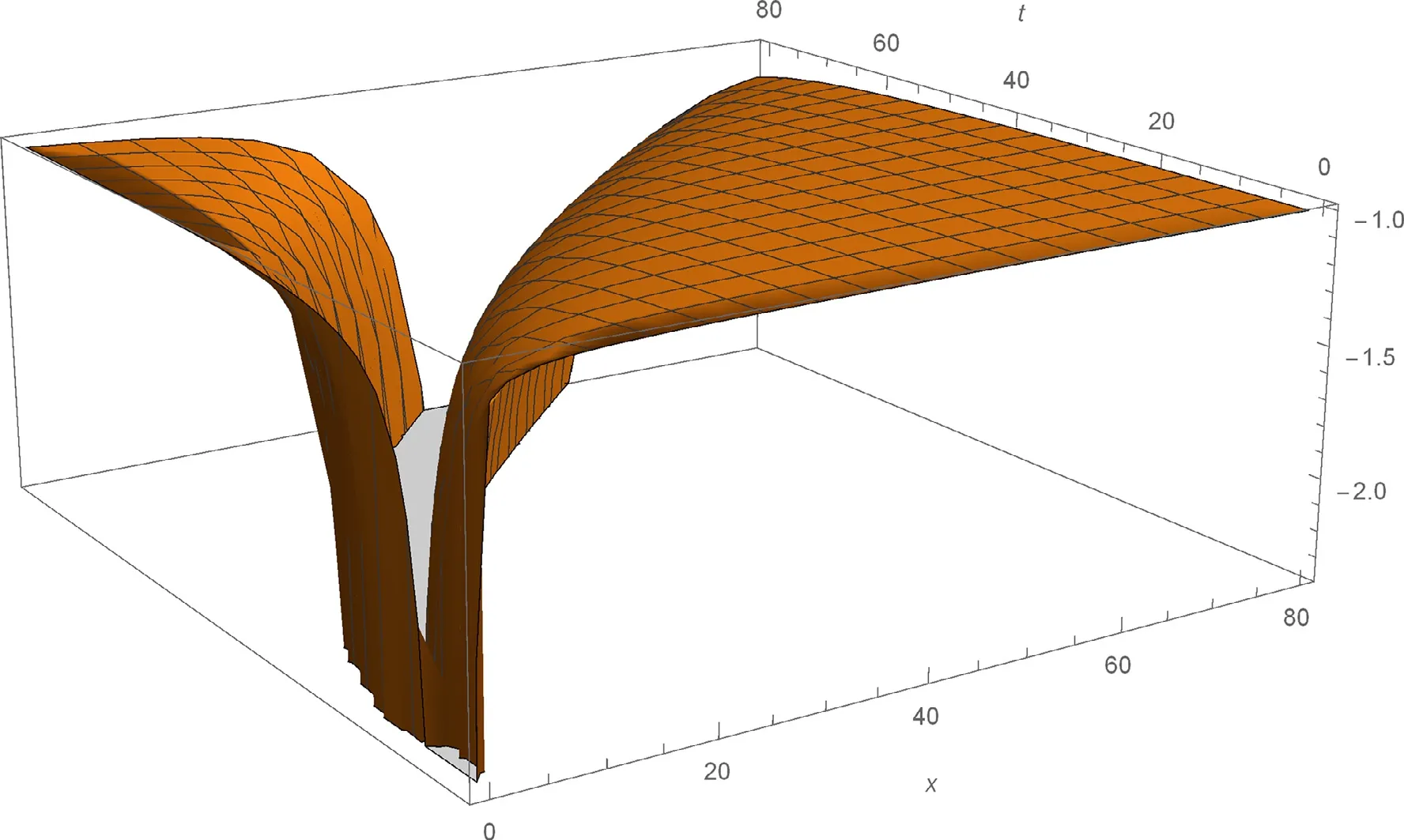
Fig. 9. 3D plot of the solitary wave solution v 3 ( x, t ) of Eq. (2) for a 0 = 0. 5 , b = 0. 7 , µ= 0, C = 1 , λ= 0. 1 , α = 0. 75 , β = 0. 5 .
The solutionsu1(x,t),v2(x,t) andv3(x,t) of Eq. (2) are simulated as traveling wave solutions for various values of the physical parameters in Figs. 5 -9 . Figs. 5 and 6 show solitary wave solutions of Eq. (2) . 3D plot of the obtained solutionu1(x,t) is given fora0= 0. 5 ,b= 0. 7 , µ= 1 ,C=1 , λ= 3 , α= 0. 75 , β= 0. 5 . Fig. 6 also illustrates the same solution with 2D plot for 0 ≤x≤ 10 att= 1 . Figs. 7 and 8 show periodic wave solutions of Eq. (2) . 3D and 2D plots of the obtained solutionv2(x,t) andv2(x, 1) are given fora0= 0. 5 ,b= 0. 7 , µ = 2,C= 1 , λ = 1 , α = 0. 75 , β = 0. 5 ,respectively. From Fig. 8 , we can see that the wave amplitudes go to infinity and the wavelengths increase when x approaches to infinity. Fig. 9 shows solitary wave solutionv3(x,t) of Eq. (2) . 3D plot of the obtained solutionv3(x,t)is given fora0= 0. 5 ,b= 0. 7 , µ = 0,C= 1 , λ = 0. 1 , α =0. 75 , β= 0. 5 . Note that the 3D graphs describe the behavior ofuandvin spacexat timet, which represents the change of amplitude and shape for each obtained solitary wave solutions. 2D graphs describe the behavior ofuandvin spacexat fixed timet= 1 . All graphics in figures are drawn by the aid of Mathematica 10.
5.Conclusion
In the present paper, the space and time fractional Broer-Kaup and approximate long water wave equations with the conformable fractional derivative are considered. By using the exp (-φ(ξ)) expansion method new approximate analytic solutions are obtained. The new analytical solutions obtained in this paper have not been reported in the literature so far.This method is useful in solving wide classes of conformable nonlinear fractional differential equations.
杂志排行

Journal of Ocean Engineering and Science的其它文章
- Development of current-induced scour beneath elevated subsea pipelines
- Optimization approach for a climbing robot with target tracking in WSNs
- The effect of gravity and inclined load in micropolar thermoelastic medium possessing cubic symmetry under G-N theory
- Efficient numerical scheme based on the method of lines for the shallow water equations
- Comparing the force due to the Lennard-Jones potential and the Coulomb force in the SPH Method
- Iterative algorithm for parabolic and hyperbolic PDEs with nonlocal boundary conditions