Joint optimization of sampling interval and control for condition-based maintenance using availability maximization criterion

LI Xin,CAI Jing,*,ZUO Hongfu,LIU Ruochen,CHEN Xi,and GUO Jiachen

1.College of Civil Aviation,Nanjing University of Aeronautics and Astronautics,Nanjing 211106,China;

2.School of Automobile and Traffic Engineering,Jiangsu University of Technology,Changzhou 213001,China;

3.Shanghai Aircraft Customer Service Co.,Ltd.,Shanghai 200241,China

1.Introduction

Recently,many critical systems or components of military and civil industry operating in severe environment experience the deterioration with usage and age.An effective method is taking appropriate preventive maintenance(PM)to avoid grave consequences led by serious degradation or failure of the system.Over the past few decades,a variety of models have been proposed for PM.The conventional PM models can be generally classified as the age based replacement model[1–3],the block replacement model[4,5]and the periodic maintenance model[6,7].In the age-based replacement model,historical statistics and cost information are needed to obtain the optimal replacement timeTc.If there is no failure occuring until the predetermined ageTc,preventive replacement should be carried out.If the system fails before the timeTc,replacement should be taken immediately.The block replacement policy requires periodic preventive replacement at uniformly-spaced timekTr( fixedTr,k=1,2,...).The periodic maintenance model is a time-dominated PM method,in which periodic repair should be taken for the systems or components.Although the aforementioned methods are simple and easy to implement,the condition monitoring information of the system in the operational process has not been taken into consideration,leading to inaccuracy failure prediction,lower equipment availability and higher maintenance cost.

In condition-based maintenance(CBM),the real-time monitoring data is used for monitoring and diagnosis of the system,then the degradation situations of the system are assessed,after which the arrangements of maintenance time and maintenance projects can be made.Compared with the traditional models,establishing reasonable and implementing effective CBM can considerably reduce the unnecessary PM measures,thus significantly reducing maintenance costs and improve equipment availability[8].In many practical applications of CBM,the operational states(healthy or unhealthy)cannot be observed directly[9].In literature,three types of statistical approaches exist to model the degradation process based on the condition monitoring information:(i)stochastic filtering-based model[10];(ii)covariate based hazard model[11,12];(iii)hidden Markov model(HMM)[13,14].Stochastic models use the unobservable states and the variables related to observable state to establish the state space model.In the covariate based risk model,the degradation is caused by the covariates.These covariates change randomly in the process of system deterioration.The HMM usually includes two random processes,one unobservable Markov chain reflecting the real degradation system state,and one observable Markov process representing the observable condition monitoring information.Among these approaches,HMM is more popular in health management,reliability analysis and CBM decision-making[14–16].To overcome the deficiency of exponential sojourn time distribution in HMM,the sojourn time in each operational state is not restricted by exponential distribution in hidden semi-Markov model(HSMM)[17].Recently,some extensions,such as Gaussian distribution and Erlang(2,λ)distribution,have been considered in HSMM[18,19],which still has limited applications.The change of shape parameter and scale parameter in Erlang distribution can approximate almost all of the continuous distributions,such as exponential,Weibull and Gamma distribution[20].Therefore,we consider a general HSMM with Erlang distribution of the sojourn time in hidden states to model the deterioration of the system.

Selecting the most appropriate time to stop the system and take maintenance measures is the key to improving the availability of equipment and reducing the maintenance cost.The multivariate exponentially weighted moving average(MEWMA),Hotelling’s T2,¯X,(I(individuals),MR(moving range))and multivariate cumulative sum(MCUSUM)control chart are used in industry to determine the stopping time.However,these non-Bayesian methods are not the optimal.The cost minimizationis considered in most of the Bayesian models as the criterion for optimizing the maintenance policy[21–25],while in many practical applications,there are more cost parameters than time parameters,and it is more difficult to obtain the cost parameters with higher sensibility.Compared with the traditional cost minimization models,availability maximization models are preferable in practical applications because the time parameters are fewer and easier to be obtained than other parameters[26].

Surprisingly,availability maximization was selected as the objective for maintenance optimization in quite limited literature[26–29].It is noted however,the aforementioned models assume the degradation processes of the system are described as a three-state HMM.To some extent,this assumption does not conform to the real applications.Maintenance optimization models using HSMM are consider-ably more complicated when compared to the maintenance models based on HMM.

The remainder of the paper is organized as follows.In Section2,an HSMM with general Erlang sojourn time distribution is employed to model the deterioration of the system.The CBM availability maximization is developed using the Bayesian approach.In Section 3,an effective computational algorithm is designed to find the optimal parameters.In Section 4,the proposed approach is illustrated by a case study.Section 5 provides concluding remarks.

2.Model formulation

2.1 Assumption and notation

Assumptions in the optimization model are listed as follows.

(i)The system deterioration process is monotonic,i.e.,the system cannot transit from unhealthy state to healthy state without PM or replacement actions.

(ii)The sojourn time in each hidden state follows general Erlang distribution.

(iii)The observations in the hidden states follow multivariate normal distribution.

(iv)Only the failure state is observable.

(v)After full inspection,PM or failure replacement,a new system cycle will start.

The following notations are used in this paper:

P:Transition probability matrix.

S:The state space of HSMM.

Δ:Sampling interval.

Δ∗:Optimal sampling interval.

ykΔ:Observation vector at sampling epoch kΔ.

Q:Instantaneous transition rate matrix.

¯Π:Fixed control limit.

Π∗:Optimal control limit.

Πk(i):The posterior probability that the system is in state i.

CL:The system cycle length.

UT:The system uptime in one cycle.

R(t|Πk):Conditional reliability function of system at sampling epoch kΔ.

Θ:The enlarged state space of HSMM.

TI:Full inspection time.

TPM:Preventative maintenance time incurred after full inspection.

TF:Replacement time incurred when system fails.

2.2 Hidden semi-Markov deterioration process

To develop an effective maintenance model,we first assume that the deterioration of the system can be described by a three-state HSMM[20],the state space of which is S={0,1,2}:state 0(unobservable good or healthy state),state 1(unobservable warning or unhealthy state)and state 2(observable failure state).Denote yΔ,y2Δ,...,ykΔ∈ Rdthe d-dimension observation data,thus ykΔconditional on the state x has d-dimension multivariate normal distribution with Nd(µx,Σx),x=0,1,and the probability density function(PDF)is given by

where µ0,µ1∈ Rd,Σ0,Σ1∈ Rd×dare unknown obser-vation parameters.

The schematic diagram of the state transition is shown in Fig.1. The transition probability matrix is P =[pij](i,j∈S),where pijrepresents the probability that the system transits to state j after leaving state i.

Fig.1 Schematic for system state transition of the 3-state HSMM

Generally,the transition probability matrix of the system is assumed as

where p01+p02=1.

Instead of the exponential sojourn time distribution assumption in HMM,we assume that in state i for i=0,1,the sojourn time in the hidden states follows Erlang distribution,the PDF and the cumulative distribution function(CDF)are respectively given by

where ki∈ N+is the shape parameter,and λ ＞ 0 is the rate parameter.The change of parameters in Erlang distribution can approximate almost all of the continuous distributions,including the Gaussian distribution used in HMM,thus the Erlang distribution is more general and applicable to model the system deterioration process.

Suppose that k1phases in state 0 and k2phases in state 1.Thus,the new state space is Θ={K1,K2,K3},where K1={1,...,k1}represents the set of healthy states,K2={k1+1,...,k1+k2}represents the set of unhealthy states,and K3={k1+k2+1}represents the failure state.For a three-state HSMM,the instantaneous transition rate matrix Q=(qij)i,j∈Z[20]is given by

The Kolmogorov backward differential equations can be used to obtain the transition probability Pij(t):

For example,when k1=k2=2,the state transition is illustrated in Fig.2.The HSMM with Erlang distribution in each hidden state essentially is the multi-state Markov process.

Fig.2 State transition of HSMM

2.3 CBM availability maximization optimization

The posterior probability that the system is in the warning state provides enough information for maintenance decision-making in Markov decision process[23,25,28].The conventional posterior probability statistic defined in HMM is given by

where ξ is the failure time of the system,ξ=inf{t?0 ∶Xt=2}.

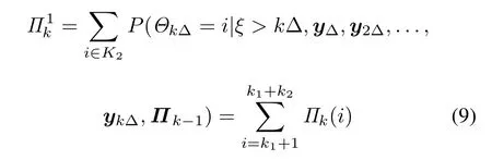
However,this posterior probability statistic is inapplicable in HSMM due to the enlarged state space. The posterior probability that the system is in state i(1≤i≤k1+k2)given the observation data yΔ,y2Δ,...,ykΔ∈ Rdat sampling time kΔ is defined as

Further,the posterior probabilitycan be defined as

For fixed¯Π∈(0,1)and Δ,the posterior probability vector Πkis updated at each decision epoch.At the sampling time kΔ,if,no actions will be taken and the system will continue running.If,the system should be stopped and full inspection should be taken to determine whether the system is in the healthy state or not,for which the inspection time is TI.The system may be found in unhealthy state with the probabilityor in healthy state with the probability.After inspection,if the system is found in healthy state,it will be left operational with some small maintenance adjustments and calibration,such as cleaning and lubricating for the mechanical components.After the small adjustments,the system is assumed to be in initial healthy state.Compared with PM action,the time of small adjustments can be negligible.This assumption is reasonable and has been used in many applications[21,24,30–33].If the system is found in the unhealthy state,PM measures will be taken with the maintenance time TPM.Ifdoes not exceed the fixed controllimit¯Π but the system still fails,i.e.,a random failure occurs, the failure replacement measures should be performed immediately,and the corresponding replacement time is TF.

Different from the cost minimization in Akram[22],the availability maximization criterion is considered in this paper.By renewal theory,the optimal values of Π∗∈ [0,1]and Δ∗with availability maximization can be obtained by

where UT and CL denote respectively the cycle system uptime and the cycle length,and term E(·)denotes the expectation operator.

Let T1be the time whenfirstly exceeds the control limit¯Π:

Thus the system uptime in a cycle is

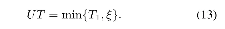
The cycle length is given by

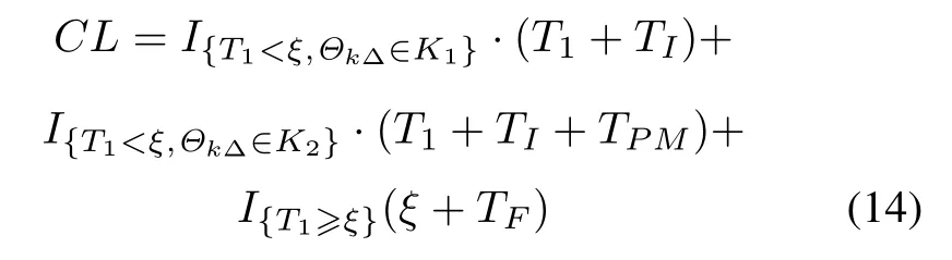
where

Next,we design an effective algorithm to determine the optimal decision variables(Π∗,Δ∗)and calculate the average availability g(¯Π,Δ).

3.Computational algorithm

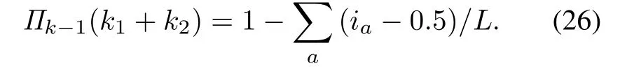
We design an algorithm in the semi-Markov decision process(SMDP)framework to find the optimal parameters.The control limit is used to determine the stopping time,and the sampling interval is used to determine when to collect data.Firstly,we need to discretize interval[0,1],the state space of Πk(i)defined in(8).At present,there are several kinds of discretization methods of the state space,such as equally or unequally-spaced intervals.We have found that equally spaced intervals discretization can lead to better convergence results.It is sufficient to choose L=30 as the number of subintervals to provide effective accuracy.For L=30,we define the SMDP is in state,i.e.,if simultaneously,the updated Πk(1)lies in the interval[(i1-1)/L,i1/L],Πk(2)lies in the interval[(i2-1)/L,i2/L],...,and Πk(k1+k2-1)lies in the intervalIf,full inspection should be performed,the SMDP is defined to bein state(j,I).The SMDP is definedin state PM if the system is found to be in unhealthy state after full inspection.If failure occurs,we define the SMDP in state F.

After de fining the state space of SMDP,we further define the following quantities:

vi:the relative value until the next decision epoch given the current state i∈S.

ci:the expected uptime until the next decision epoch given the current state i∈S.

τi:the expected sojourn time until the next decision epoch given the current state i∈S.

P(k-1,i),(k,j):the probability that at the sampling epoch kΔ the system will be in state j∈ S given the sampling epoch(k-1)Δ the state is i∈ S.

According to the theory of SMDP,the expected average availability g(¯Π,Δ)can be obtained[34]by

Thus the optimal Π∗and Δ∗can be obtained by

which is acquired by solving the linear equations defined in(15)iteratively with different control limits Π¯and sampling intervals Δ.Next,we will deduce the updated posterior probability Πk(i),transition probabilities P(k-1,i),(k,j),expected sojourn time τiand expected uptime ci.

3.1 Posterior probability computation

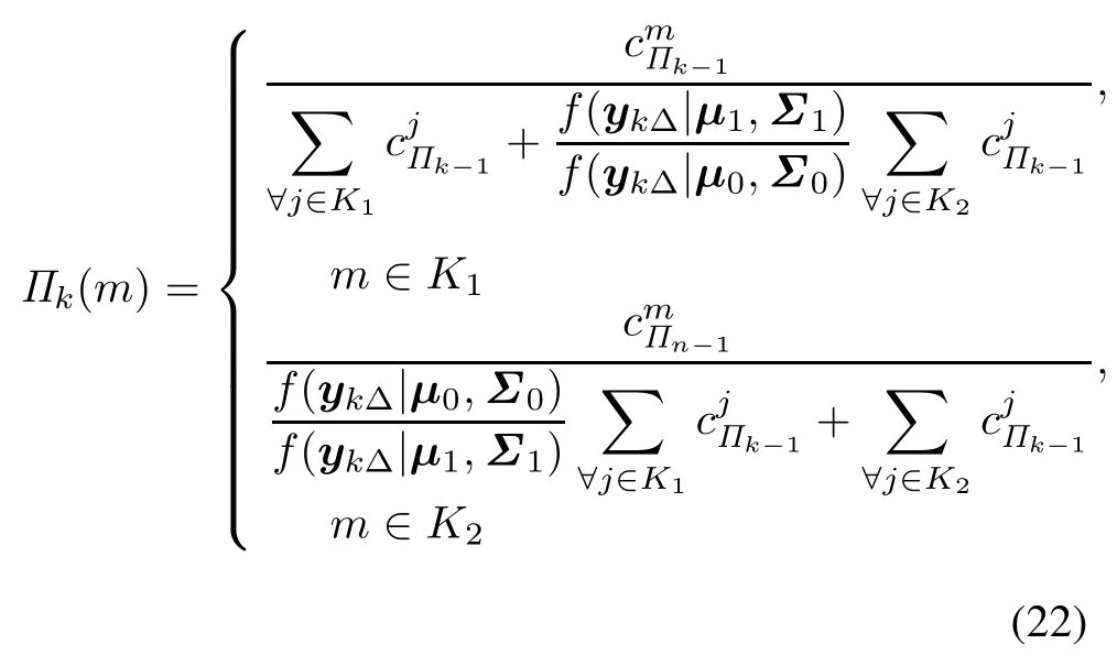
According to the Bayes’theorem,the posterior probability Πk(i)can be updated iteratively at each sampling epoch by the following formula:

From(1)we can obtain

Further,for i∈ K1,posterior probability Πk(i)is given by

and for i∈ K2,posterior probability Πk(i)is given by

Different from the assumption Σ0= Σ1made by Maiks[25],we assume Σ0/= Σ1,which is common in real maintenance practice,thus from(1)we can further obtain

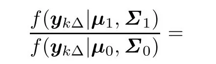
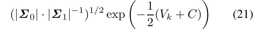
Therefore,the posterior probability can be rewritten as

3.2 Transition probabilities

In order to derive the explicit expressions of quantities in the SMDP,we need to deduce the conditional reliability function(CRF) first.

Lemma 1For t?0,the CRF of the system at sampling epoch kΔ is given by

ProofSuppose ξ＞ kΔ,then for t?0,the CRF is given by

Lemma2Foreachstate,the transition probabilities are given by

where for m∈K1,

and for m∈K2,

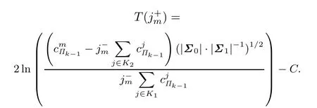
ProofFor each stateand,the transition probabilities are given by

For m∈K1,the probabilitycan be obtaine

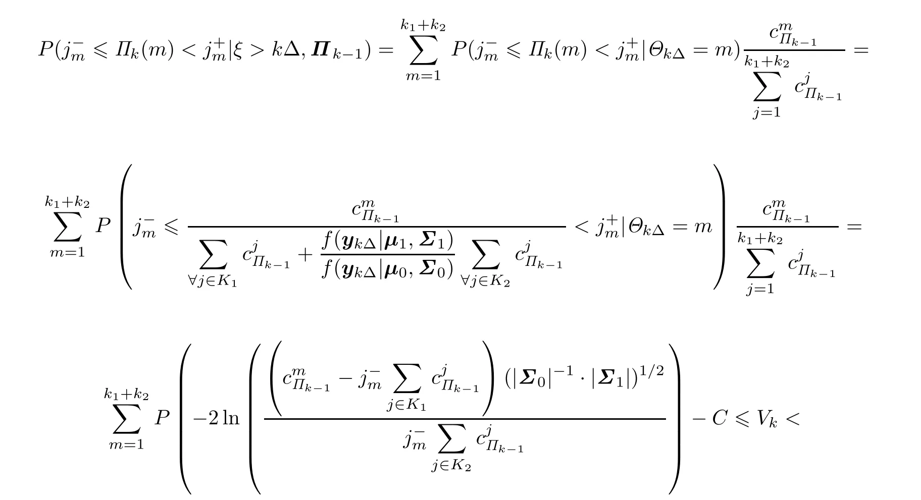
Similarly,for m ∈ K2,the probabilitycan be obtained by

Therefore,transition probabilities are given by(24).?

Assume at sampling time(k-1)Δ,SMDP is in state(i1,i2,...,ik1+k2-1).The posterior probability vectorcan be approximately calculated by the mid-point which is given by

and

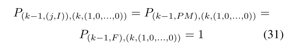
Once full inspection or failure replacement measures are performed,the state will transit to the initial healthy state,therefore the transition probabilities are given by

3.3 Expected sojourn times

If after full inspection,the system is in healthy state,the expected sojourn time is given by

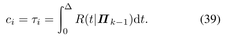
If the system is in state PM,the expected sojourn time and expected system uptime are respectively given by

If the system is in state F,the corresponding expected sojourn time is given by

3.4 Expected system uptimes

If after full inspection,the system is in healthy state,the expected system uptime is given by

If the system is in state PM and state F,the expected system uptimes are given by

In Section 4,the whole procedure will be illustrated by a case study.

4.Experimental results

4.1MCMC simulation

In order to optimize the control limit and sampling interval,Markov chain Monte Carlo(MCMC)is used to generate the simulated data.The flow chart of MCMC is depicted in Fig.3.

Fig.3 Flow chart of MCMC simulation

Suppose k1=3,k2=2 and λ=0.3.The transition probability p01=0.8 and p02=0.2.The observations yΔ,y2Δ,...,ykΔ∈ R2are obtained from the condition monitoring data,which follows N2(µ0,Σ0)in healthy state and follows N2(µ1,Σ1)in unhealthy state,where

Maintenance time parameters are given by TI=1 h,TPM=5 h and TF=30 h.Thus,the instantaneous transition rates matrix is given by

Different combinations of¯Π∈(0,1)and Δ∈(0,2]are chosen with the step of 1×10-4.Meanwhile,the subinterval number L=30 is selected to divide the interval[0,1].

We calculate the optimal control limit Π∗and sample interval Δ∗with the objective of availability maximization.The results are shown in Table 1.Next,the proposed method will be compared with other policies.

Table 1 Results for optimal Bayesian control chart basedon HSMM

4.2 Comparison of optimal parameters with HMM

As the HSMM is the extension of HMM,we first compare the proposed approach with that based on HMM.The results are shown in Table 2.

Table 2 Results for optimal Bayesian control chart based on HMM

As illustrated in Table 2,the average availability obtained based on HMM is 0.498 3,which is lower than the results of the proposed method based on HSMM.

4.3 Comparisons with other control charts

Further,we use the same model parameters of HSMM in subsection 4.1 to simulate 20 failure histories and 20 suspension histories.Fig.4 shows the bivariate observations for a failure history.Fig.5 represents the bivariate observations for a single suspension history.

Taking the failure history in Fig.4 as an example,we first illustrate the multivariate Bayesian control charts based on HMM and HSMM.The posterior probability is updated by(22),and the Bayesian control charts are shown in Fig.6.

Fig.4 Bivariate observations for a failure history

Fig.5 Bivariate observations for a suspension history

Fig.6 Bayesian control chart using different Markov models

From Fig.6,using the proposed method in this paper,the posterior probability firstly exceeds the control limit at the 21st sampling epoch,while using the method based on HMM,the optimal stopping time should be at the 23rd sampling epoch,which verifies that the proposed method is able to detect the change of system from healthy state to unhealthy state much earlier than the method based on HMM.

Then we compare the proposed approach with other approaches.The age-based replacement policy is an effective method for maintenance decision-making[27].In this policy,the optimal preventive replacement time τ satisfies

where R(t|Π0)is the CRF at the initial moment andis the hazard rate function.

Recently,other control charts such as Hotelling’s T2[35],MEWMA and MCUSUM have been used in the maintenance policy extensively[36].For Hotelling’s T2chart,the statistic T2is given by

where

The control statistic Tnin MEWMA chart is given by

The control statistic Snin the MCUSUM chart is given by

We now use the 20 failure histories and 20 suspension histories to verify the proposed approach.If the failure occurs before the chart signals,the corrective maintenance(CM)should be performed.If the chart signals occur before the failure,i.e.,true alarm occurs,the PM should be performed.Otherwise,false alarm will occur.We apply the above methods to the historical data,the results are shown in Table 3.

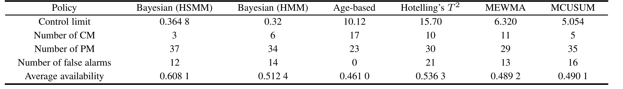
Table 3 Comparisons with other methods

Table 3 shows that using the same maintenance time parameters,the optimal average availability calculated by the proposed method is equal to 0.608 1.Comparing the Bayesian control chart based on HSMM with other approaches,the expected average availability obtained by our method is the largest,while that from the age-based replacement policy is lower than other methods due to ignorance of the condition monitoring information.The number of PM obtained by the proposed approach is also the largest,which indicates the Bayesian control chart based on HSMM can detect the state change accurately.

5.Conclusions

In this paper,we have considered a Bayesian control scheme based on HSMM for CBM availability maximization.The general Erlang sojourn time distribution is considered.Based on HSMM,an optimal Bayesian control scheme with availability maximization criterion is developed.The optimal sampling interval and control limit are solved in the SMDP framework.The comparison with the Bayesian control scheme based on HMM,age based replacement policy,Hotelling’s T2,MEWMA and MCUSUM control charts indicate that the proposed approach can achieve higher average availability and detect the system change accurately. The method presented in this paper can make full use of the multivariate condition moni-toring information.Using the optimization model we propose,the maintenance decision maker can decide when to collect the condition monitoring data,as well as when to stop the system and initiate PM actions.

In this research,we have considered the general HSMM and the Bayesian control chart method with the objective of availability maximization.The mean residual life can be deduced in the future research.On the basis of the promis-ing results,two or multiple sampling intervals can also be considered based on HSMM for CBM cost minimization or availability maximization,which is a suitable topic for the future work.

Acknowledgements

The authors are grateful to Prof.Viliam Makis in University of Toronto for discussions.

[1]CHRISTER A H.Comments on finite-period applications of age-based replacement models.IMA Journal of Management Mathematics,1986,1(2):111–124.

[2]CHEN M,MIZUTANI S,NAKAGAWA T.Random and age replacement policies.International Journal of Reliability,Quality and Safety Engineering,2010,17(1):27–39.

[3]LI P,WANG W,PENG R.Age-based replacement policy with consideration of production wait time.IEEE Trans.on Reliability,2016,65(1):235–247.

[4]SCARF P A,DEARA M.Block replacement policies for a two-component system with failure dependence.Naval Research Logistic,2003,50(1):70–87.

[5]KE H,YAO K.Block replacement policy with uncertain lifetimes.Reliability Engineering&System Safety,2016,148:119–124.

[6]PARK D H,JUNG G M,YUM J K.Cost minimization for periodic maintenance policy of a system subject to slow degradation.Reliability Engineering&System Safety,2000,68(2):105–112.

[7]CERTA A,ENEA M,GALANTE G,et al.A multi-objective approach to optimize a periodic maintenance policy.International Journal of Reliability,Quality and Safety Engineering,2012,19(6):1240002.

[8]JARDINE A K S,LIN D,BANJEVIC D.A review on machinery diagnostics and prognostics implementing condition based maintenance.Mechanical Systems and Signal Processing,2006,20(7):1483–1510.

[9]LEE J,WU F,ZHAO W,et al.Prognostics and health management design for rotary machinery systems-reviews,methodology and applications.Mechanical Systems and Signal Processing,2014,42(1):314–334.

[10]WANG Z,HU C,WANG W,et al.A case study of remaining storage life prediction using stochastic filtering with the influence of condition monitoring.Reliability Engineering&System Safety,2014,132:186–195.

[11]MAKIS V,JARDINE A.Optimal replacement in the proportional hazards model.INFOR:Information Systems and Operational Research,1992,30(2):172–183.

[12]KUMAR D,KLEFSJO B.Proportional hazards model:a review.Reliability Engineering&System Safety,1994,44(2):177–188.

[13]KIM M J,MAKIS V,JIANG R.Parameter estimation in a condition-based maintenance model.Statistics&Probability Letters,2010,80(21):1633–1639.

[14]SI X,WANGW,HUC,et al.Remaining useful life estimation-a review on the statistical data driven approaches.European Journal of Operational Research,2011,213(1):1–14.

[15]YANG S,QIU J,LIU G,et al.Optimization of dynamic sequential test strategy for equipment health management.Journal of Systems Engineering and Electronics,2012,23(1):71–77.

[16]ZHAO J,DENG J,YE W,et al.Combined forecast method of HMM and LS-SVM about electronic equipment state based on MAGA.Journal of Systems Engineering and Electronics,2016,27(3):730–738.

[17]YU S.Hidden semi-Markov models.artificial Intelligence,2010,174(2):215–243.

[18]JIANG R,KIM M J,MAKIS V.Maximum likelihood estimation for a hidden semi-Markov model with multivariate observations.Quality and Reliability Engineering International,2012,28(7):783–791.

[19]LIU Q,DONG M,LV W,et al.A novel method using adaptive hidden semi-Markov model for multi-sensor monitoring equipment health prognosis.Mechanical Systems and Signal Processing,2015,64/65:217–232.

[20]KHALEGHEI A,MAKIS V.Model parameter estimation and residual life prediction for a partially observable failing system.Naval Research Logistics,2015,62(3):190–205.

[21]LI X,CAI J,ZUO H,et al.Optimal cost-effective maintenance policy for a helicopter gearbox early fault detection under varying load.Mathematical Problems in Engineering,2017,2017:1–16.

[22]KHALEGHEI A.Modeling,estimation,and control of partially observable failing systems using phase method.Toronto,Canada:University of Toronto,2016.

[23]KIM M J,MAKIS V.Joint optimization of sampling and control of partially observable failing systems.Operations Research,2013,61(3):777–790.

[24]KIM M J,JIANG R,MAKIS V,et al.Optimal Bayesian fault prediction scheme for a partially observable system subject to random failure.European Journal of Operational Research,2011,214(2):331–339.

[25]MAKIS V.Multivariate Bayesian control chart.Operations Research,2008,56(2):487–496.

[26]JIANG R,KIM M J,MAKIS V.Availability maximization under partial observations.ORS pectrum,2013,35(3):691–710.

[27]BARLOW R,HUNTER L.Optimum preventive maintenance policies.Operations Research,1960,8(1):90–100.

[28]JIANG R,KIM M J,MAKIS V.A Bayesian model and numerical algorithm for CBM availability maximization.Annals of Operations Research,2012,196(1):333–348.

[29]MAATOUK I,CHATELET E,CHEBBO N.Availability maximization and cost study in multi-state systems.Proc.of IEEE Annual Reliability and Maintainability Symposium,2013:1–6.

[30]NADERKHANI F,MAKIS V.Economic design of multivariate Bayesian control chart with two sampling intervals.International Journal of Production Economics,2016,174:29–42.[31]LIN C,MAKIS V.Optimal Bayesian maintenance policy and early fault detection for a gearbox operating under varying load.Journal of Vibration and Control,2016,22(15):3312–3325.

[32]JAFARI L,MAKIS V.Optimal lot-sizing and maintenance policy for a partially observable production system.Computers&Industrial Engineering,2016,93:88–98.

[33]JIANG R,YU J,MAKIS V.Optimal Bayesian estimation and control scheme for gear shaft fault detection.Computers&Industrial Engineering,2012,63(4):754–762.

[34]TIJMS H C.A first course in stochastic models.Chichester:Wiley,2001.

[35]FARAZ A,CHALAKI K,SANIGA E M,et al.The robust economic statistical design of the Hotelling’sT2chart.Communications in Statistics-Theory and Methods,2016,45(23):6989–7001.

[36]ALYAA,MAHMOUDMA,HAMEDR.The performance of the multivariate adaptive exponentially weighted moving average control chart with estimated parameters.Quality and Reliability Engineering International,2016,32(3):957–967.