Grey interpolation approach for small time-lag samples based on grey dynamic relation analysis

WANG Junjie,DANG Yaoguo,XU Ning,and DING Song

1.College of Economics and Management,Nanjing University of Aeronautics and Astronautics,Nanjing 211100,China;2.College of Management Science and Engineering,Nanjing Audit University,Nanjing 211815,China

1.Introduction

The social and economic statistical data of developed countries normally keep a smooth trend,while the data in developing countries are usually in different tendencies.A small sample is commonly utilized by the analysts when one may wish to forecast or evaluate the economy in a developing country.In addition,one or more data in a small sample may be lost or abnormal values because of the distinct statistical calibers.For example,one may wish to investigate the tendency of investments in fixed assets of Qingdao which is an important city in Shandong province.However,the data in 2006 cannot be obtained from the government website.In order to analyze the sequences having missing data or outliers,a number of scholars proposed some approaches for non-equidistant sequences to analyze them.Meanwhile,many interpolation models were put forward to producea reasonable value for a missing or abnormal datum.

A fast and exact method using projected convolution was proposed for non-equidistant grids by Hackbusch[1].Sampling patterns which were composed of the zeros of sine-type functions were considered as well as the local and global convergence behavior of the sampling series to deal with the non-equidistant sampling series in signal processing by Boche and Monich[2].A finite difference approach having non-uniform meshes for calculating nonlinear fractional differential equations was presented to solve the less smooth problems[3].A novel approach integrating Burt-Adelson’s Laplacian pyramids with lifting schemes was presented for the non-equispaced data[4].In addition,a number of grey forecasting models which was utilized for the small sample data were developed for the non-equidistant time series.Xie et al.[5]presented a new grey prediction model for a non-homogeneous index sequence to broaden the scope of grey models.In order to reduce the effects of empirical mode decomposition,a new method which was motivated by the non-equidistance grey model was presented by He et al.[6].A fractional order grey forecasting model that was effective for non-equidistant time series was proposed by Shen et al.[7].A rolling optimum method used for generating the background sequence in a grey system was derived to deal with the multiple non-equidistant sequences[8].

The interpolation approaches are also executed to produce a relational value for analyzing the non-equidistant data.A novel method which integrates the state-space matrix interpolation and the least-squares approximation is put forward to produce a linear parameter-varying[9].Shekhtman’s method is improved to find a sequence of interpolation sites which could make the corresponding Lagrange interpolations converge to them[10].A combination of the piecewise linear interpolation function and Newton interpolation method is presented to generate the unknown background value for improving the prediction accuracy[11].A novel interpolation technique called grey distance information approach for small samples is put forward according to the grey relational theory and norm theory[12].To evaluate some simulation systems having small sample data,a grey confidence interval is proposed which could generate small samples[13].

As discussed above,the general methodology used for the time series sequence with the missing data,which can also be regarded as a non-equidistant sequence,is normally not suitable for the small sample data because of the statistical rule as well as the interpolation technique.The grey theory,which was proposed by Deng[14]in the early 1980s,is a powerful tool to analyze the systems with limit information.A series of grey models for forecasting and evaluating the non-equidistant sequences are put forward as introduced above.However,the overwhelming majority of these models,whose basic thoughts of dealing with the missing value are linear generation according to the length of time,ignore the dynamic trend and the connection with other relevant sequences.To improve the accuracy of the interpolated values,the relational sequences should be considered for obtaining more information to produce the missing data because the information of one small sample is limited.

In order to address the aforementioned shortcomings,an interpolation approach based on the grey dynamic incidence model containing a time lag specified by t,denoted as GDIM(t),is presented in this paper.The unknown actual value of a missing or abnormal datum is a grey number whose definition is given in definition 6.A novel grey incidence model based on dynamic relation analysis which considers the positive and negative connections between the two sequences is proposed.A time lag is used when calculating the dynamic connections between the two sequences.A series of constraints obtained from the novel grey incidence model are utilized to design two programming problems for determining the upper and lower bounds of the grey number.

The remainder of this paper is organized as follows.In the next section,two perspectives are described for using a grey number in practical applications.In addition,the procedure and importance of this new grey interpolation approach are explained.Within Section 3,the GDIM(t)model utilized in the novel grey interpolation model is constructed.Two programming problems used for producing the upper and lower bounds of the unknown grey number which represents the missing or abnormal value are given as well as the solutions of them. Subsequently, in Section 4,a case study involving a sequence with an outlier about the agriculture environment is utilized for demonstrating how the new grey interpolation approach can be applied in practice.

2.Procedure and potential applications of the proposed interpolation approach

The grey number is the basic element in grey systems. Over the years, most of the theoretical developments and practical applications of grey numbers have fallen under the domain of using a given grey number. The existing researches focus on the methods for evaluating or forecasting a system with known grey numbers [15 – 18]. To broaden the scope of applications of grey numbers, a new perspective of applying a grey number to an uncertain system is proposed in this paper. Different from the traditional ways of using a grey number, the grey number is produced by two programming problems in this work rather than given.

In some real life situations,one may understand that an unknown number in a sequence is a grey number.However,the reliable interval of the unknown datum is not given.To evaluate or forecast the systems having one or more such values,a novel grey interpolation method is carried out to narrow the range of the grey number for a better evaluation or prediction.In this section,the procedure of implement-ing the proposed grey interpolation approach for producing a grey number is portrayed in Fig.1.In practices,two potential applications for solving different problems are described in Fig.2.

As depicted in Fig.1,the procedure of the proposed grey interpolation approach considering time lags for small sample data consists of seven steps.The highlights of this research fall under the domain of Step 3 and Step 5.The main idea of constructing a grey dynamic incidence model in Step 3 for determining the relational factors is portrayed in Fig.1.As depicted in Fig.1,the novel grey dynamic incidence model,which is an improvement of the traditional grey incidence models[19–22],considers the positive and negative relationships and the time lag t between the two sequences.In Step 5,the programming problem for optimizing the upper and lower bounds of the unknown grey number are established according to the relationships among the factors determined in Step 2.Then,the minimum upper bound and maximum lower bound satisfying all the constraints can be obtained.Finally,the new sequence with the interpolated data is utilized for evaluating and forecasting in practices.

Fig.1 Procedure of the grey dynamic incidence model and grey interpolation approach

In practices,a large number of data can be collected while a part of them which constitute a small sample are effective for research.Sometimes,a small sample datum can be obtained.The analyst may find that one or more values of the small sample data are missing or outliers which would affect the research.

As just mentioned,two fundamental ways in which the novel grey interpolation approach can be utilized for addressing small samples are:

(i)For a non-equidistantsmall sample,ascertain the connections with other related factors to construct the constraints for producing a reasonable value;

(ii)For an equidistant small sample with one or more abnormal values,generate an effective value for replacing the outlier.

These two situations that could occur in a study based on small samples are depicted as the upper and lower diagrams in Fig.2,respectively.

Fig.2 Two potential application of the novel grey interpolation method

3.Design of the novel grey interpolation approach

The novel grey interpolation method is utilized for determining the missing data or correcting the outliers in a small sample.To accomplish this,a grey dynamic incidence model containing a time lag specified by t,called GDIM(t),is constructed in Section 3.1.Then,within Section 3.2,two programming problems according to the connections obtained from the GDIM(t)model are given for calculating the bounds of the grey number representing the missing or abnormal value.The solutions for estimating the grey number according to the particle swarm optimization(PSO)methodology are summarized in Section 3.3.

3.1 Construction of the grey dynamic incidence model

Within this section,trigonometric functions are utilized for determining the trend of the sequence at each data point in the GDIM(t)model.The definitions for the key components of the two main parts called measurement factor and judgement factor which constitute the GDIM(t)model as well as the formulae of the GDIM(t)model containing the time lag t are given in Section 3.1.

definition 1Assume thatis an original set of data with the kth observation value(k=1,2,...,n)for an object i.Thenis called the original sequence of.If k stands for the time order,is the original value ofat time k,andis the original time series sequence of

definition 2Standardization:From definition 1,letbe theoriginal time series sequence of.Then,letanddenote the average value and standard deviation ofrespectively.Then,...,xi(n))is called the standardized time series,for which

From this point onwards,the definitions containing the new theoretical developments in the grey relational analysis are based on using the standardized time series to ensure compatibility when comparing different time series.

definition 3Let Xi=(xi(1),xi(2),...,xi(n))and Xj=(xj(1),xj(2),...,xj(n))denote the standardized time series sequences ofand,respectively.Assume that the original time series as well as the standardized time series consist of values which are equally spaced in time.define an angle αi(k)and αj(k)for keeping track of the trend of Xiand Xjat time k where

definition 4Measurement factor and judgement factor:Given two standardized time series sequences Xiand Xjhaving a time lagis defined as definition 3.Let 1denote the measurement factor of the GDIM(t)model.Then,the judgement factor is given as follows:

definition 5[26] Grey dynamic incidence model:From definition 4,the final formulae for the novel grey dynamic incidence model consisting of the measurement factor and judgement factor are given as follows.

For a given time lag tij,the degree of the grey incidence at the kth data point or time k is given by

Over time k,one can obtain the array of the grey dynamic incidence:

By allowing the lag tijto change,one can obtain the matrix of grey dynamic incidence:

where a dash“-”in(3)indicates that the degree of the dynamic incidence cannot be calculated under the specified time lag tij.

3.2 Design of programming problem

As portrayed in Fig.1,the novel grey dynamic incidence model proposed in Section 3.1 is utilized to determine the related factors and the time lag.Hence,some constraints for establishing the programming problem based on the connections between the sequence with missing or abnormal values and its relational factors are designed in this section.Within Section 3.2,the for mulae using the degrees of grey dynamic incidence are given to optimize the bounds of the grey number which represents the missing datum or outlier.

definition 6Grey number:Let⊗x be a real number whose exact value is unknown.An interval of⊗x containing the upper bound⊗x+and lower bound⊗x-are given.Then,⊗x is called a grey number in grey systems.

As can be seen,the missing or abnormal datum in a given sequence is a real number whose exact value is unknown for the analysts.Hence,it is a grey number.Normally,the two values beside the unknown datum are utilized to determine the bounds of the grey number where the larger one represents the upper limit while the smaller one is regarded as the lower bound.

As described above,assume that xi(s)is the missing or abnormal value of a given sequence Xi=(xi(1),xi(2),...,xi(n)).Hence,the unknown datum xi(s)can be regarded as a grey number⊗xi(s)whose upper and lower limits areandrespectively.Actually,⊗xi(s)is equal to xi(s).It is assumed that the related factors of Xiare Xj(j=2,3,...,m)whose average degrees of grey dynamic incidence are larger than a where a∈[0.5,1]is a real number determined by an analyst according to the reality.The time lag tijbetween Xiand Xjis determined using the GDIM(t)model.Letandbe the unknown degrees of grey dynamic incidence at the(s-1)th and the sth data points with the specified time lag(k=1,2,...,s-2,s+1,...,n)are the known degrees of grey dynamic incidence under the specified time lag tij.

In order to obtain the interval of the grey number⊗xi(s),several constraints are established to limit the upper and lower bounds in(4).The first and second constraints represent the degrees of the grey incidence at the(s-1)th and the sth data points with the time lag tijbetween Xiand Xjaccording to definition 5.The third constraint is utilized to control the upper and lower limits of the grey number.In accordance with(1),andmust be less than or equal to 1.In addition,it is assumed that the unknown value satisfies the trend of its sequence and abides by the normal connections.Hence,two assumptions thatandshould be larger than the minimal degree of grey incidence over time k,denoted byare proposed to limit the grey number,respectively.In practice,an analyst may wish to enlarge the minimal value because of the high connection between two sequences.A coefficient,denoted by η,is utilized in the third constraint as shown in(4).When η is equal to 1,it indicates that the unknown degrees of grey dynamic incidence subject to the interval from the minimum degree to 1.The constraints are becoming more and more stringent as the coefficient η decreases from 1 toThe fifth and sixth constrains are the formulae ofandwhich are defined in definition 4.The two judgement factors should be equal to 1 because the sequence Xjutilized for producing the unknown value must has a high relationship with Xi.Then,the two mixed nonlinear programming problems are given as follows:

The lower limit⊗xi(s)-can be determined by(4)in which the target is the minimum value Z-.Similarly,the upper limit⊗xi(s)+can be obtained when the objectis the maximum value Z+=⊗xi(s)using the same constraints.

Notice,the value of⊗xi(s)obtained from the grey interpolation approach is a standardized number.

3.3 Solutions for the programming problems

The approach called PSO is carried out to explore the solution for the programming problems derived in Section 3.2.The basic steps for the above two programming problems according to the PSO algorithm are summarized in this section.

Let N be the repeat times of the PSO algorithm.Let P be the number of the PSO population.Let Particle denote a P-dimensional vector in which Particle(l)is the lth particle.Let Pupand Pdownbe the initial upper and lower bounds of the particles.Let Gbestbe an index to global-best position.Let Pbestbe the position of the local-best position.Let fitness(l)be the cost function of the l th particle according to the object of(4).

For(4)representing the first programming problem whose object is Min Z-=⊗xi(s),the steps are given as follows:

Step 1Initialization:For each particle l in the population where l∈{1,2,...,P}.

Initialize Pupand Pdownwith the fifth and sixth constraints in(4);

Let fitness(l)=Particle(l).

Step 2Repeat the following steps for N times:

Step 2.1For each particle l,let fitness(l)=Particle(l)iff Particle(l)satisfies the constraints given in(4),otherwise fitness(l)=Particle(l)=Pup;

Step 2.2Let

Step 2.3Update

Step 2.4For each particle l,update Particle(l)=

For the second programming problem whose object is Max Z+=⊗xi(s)subjecting to the same constraints,its solution can be obtained using the similar steps.

4.Application of the novel grey interpolation approach

Agriculture played an important role in the conventional economy in a developing country,e.g.China in the mid-1990s.The environment in the countryside became worse and worse because of the increasing use of chemical fertilizer,pesticide and insecticides.The chemical oxygen demand(COD)is utilized to measure the pollution in this section.The data of COD from 1993 to 2001 as depicted in Fig.3(a)are calculated by Liang et al.[23].The value of COD in 1997 decreases while the data in other years are in rising trend.Hence,it may be an outlier.The novel grey interpolation approach considering time lags between factors is carried out to update the abnormal value.To accomplish this,four possibly related factors,called gross annual value of agricultural production(GAP),proportion of animal husbandry(PAH),sown area(SA)and irrigation area(IA),are determined according to the existing research[23,24].Within Section 4.1,the GDIM(t)model proposed in this work is utilized for determining the relational factors and time lags.The abnormal value is corrected by using the new grey interpolation approach in Section 4.2.The novel grey interpolation method is utilized for producing the missing method.The performance of the proposed interpolation model is compared with four approaches in Section 4.3.

4.1 Analysis of the factors

In this section,the GDIM(t)model is utilized to determine the time lags between COD and its related factors.From Fig.3(a),it is reasonable to suspect that the value of COD in 1997 may be an outlier in this sequence.In order to verify this hypothesis,four possibly related factors are selected to calculate the relationships with COD.If the connection keeps the same trend in 1997, it is not an abnormal value. From Fig. 3(b), the dynamic relationships between COD and GAP keep around 0.8 which is really high.However, the degrees of grey dynamic incidence decrease in 1996 and 1997 as well as the connections between COD and SA. Hence, the value of COD in 1997 is determined to be an outlier. To correct the abnormal value in this system,the connections between COD and its possibly related factors are measured using the GDIM(t) model at different time lags. The original data of GAP, PAH, SA, and IA from 1990 to 2005 having more values than COD from 1994 to 2001 are given in Table 1 and Table 2, respectively.

Fig.3 Original data of COD and its connections with GAP and SA

Table 1 Original data of COD from 1994 to 2001

In Table 1 and Table 2,COD is marked as X1while the four factors are denoted as X2,X3,X4and X5.The units of these five sequences are million tons,billion Yuan,percents,hectares and hectares,respectively.The data in Table 2 are given by Zhang et al.[24].

The specified time lags are from-4 to 4 because the values of COD given in Table 1 are seven.The matrix of grey dynamic incidence representing the connections between COD and GAP with the changing time lags is given as follows using the GDIM(t)model after standardizing the original data.The other three matrices are not listed in this paper.The average degrees of grey dynamic incidence with different time lags are portrayed in Fig.4.In the below matrix,a dash“-”indicates that the value cannot be calculated because of the outlier in the original sequence.

Table 2 Original data of GAP,PAH,SA,and IA from 1990 to 2005

The average degrees of grey dynamic incidence can be obtained after calculating the other three matrices which are not given in this paper.The results are depicted in Fig.4.In this paper,the factor is effective if the average degree of grey dynamic incidence is higher than 0.8.From Fig.4(a),the connection between COD and GAP keeps in a high level when the time lag is 1.In Fig.4(b)and Fig.4(d),the highest degrees of grey dynamic incidence are onlyaround0.6.Therefore,the factors X2and X4cannot be utilized to calculate the correct interval of the outlier in X1.According to Fig.4(c),the highest degree of grey dynamic incidence is 0.85 when the time lag is-1.

In summary,the useful factors for producing a reasonable interval of the outlier are GAP and SA whose time lags are 1 and-1.Then,the arrays of the grey dynamic incidence for GAP and SA are given in the following table.In Table 3,is the degree of grey dynamic incidence in which tjis the time lag between Xiand Xj.The time lags have been determined in Fig.4.

Fig.4 Average degrees of grey dynamic incidence between COD and four factors

Table 3 Array of grey dynamic incidence between COD and its two related factors

4.2 Interval correction for the outlier

Within this section,the upper and lower limits of the outlier satisfying the constraints established in Section 3.2 are calculated according to the degrees of grey dynamic incidence with the time lags given in Section 4.1.

From Section 4.1,the parameters in(4)can be determined where i=1,j=2,4,s=4,k=1,2,5,6,7,and t=-1.Hence,and14In this case study,let the coefficient η be 0.95 to keep the four unknown degrees in a reliable interval because the minimum degree of grey dynamic incidence is only 0.687 which implies the connection is not very high as can be seen in Table 3.Hence,the constraints in(4)can be written as follows:

Note that the parameter k which stands for the year in the sequences of X2and X4should be the same as the year of X1.

As described after(4),in order to obtain the upper bound⊗xi(4)+and lower bound⊗xi(4)-of the grey number⊗xi(4),let Max Z+= ⊗xi(4)and Min Z-=⊗xi(4)subject to the constraints listed in(5),respectively.

The computational implementation of solutions for the above programming problem is based on Matlab R2012b according to the procedures given in Section 3.3.The results of the two programming problems are listed in Table 4 and portrayed in Fig.5.In Fig.5(a)and Fig.5(b),the number of particles,denoted by P,are 20,30,and 60,respectively.

From Fig. 5, the fitness values for different sizes of particles are coincident with each other after the repeat number is larger than 300.Hence,the results are effective.

Table 4 Results of the two programming problems

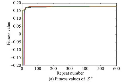
Fig.5 Fitness values of the two objects for different number of particles

The computer findings from Matlab R2012b are given in the following table.In Table 5,the fitness value is a standardized number as mentioned at the end of Section 3.2.The restored value is the original datum which is useful for the analysts.

Table 5 Results of the generated grey number

Therefore,the interval of the grey number⊗xi(4)is[5.723 2,5.733 0]which satisfies the constraints in(5).

4.3 Interval generation of the missing data

To illustrate how the novel approach can be used for a non-equidistant sequence,assume that the original value of X2in 1996 in Table 2 is unknown.Hence,the new grey interpolation approach is carried out for calculating the missing value according to the basic analysis in Section 4.1.As portrayed in Fig.4(a),the data set of COD has a high connection with that of GAP.Hence,X1which has a time lag t12with X2as given in Table 3 is determined for estimating the missing number by using the model proposed in this paper.The abnormal number of X1is corrected by 5.728which is the average value of⊗x1(4).The procedure of producing the missing data⊗x2(7)is similar to that in Section 4.2.Then,the results are given in Table 5.

In addition,in order to demonstrate the effectiveness and correctness of the proposed algorithm,four interpolation models,which are the Lagrange interpolation model[25],GM(1,1)[5],linear interpolation method,and cubic spline interpolation approach,are utilized for comparing the performance of this new model,respectively.The upper limit of⊗x2(7)is used for the comparison because it stands for the highest connections with X1.The comparison of the performances among different interpolation ap-proaches are given in Table 6.In Table 6,GIA,LaI,LiI and CSI indicate the grey interpolation approach,Lagrange interpolation model,linear interpolation method,and cubic spline interpolation approach,respectively.

Table 6 Comparison of the performances

The actual value of the unknown number is 14 015 as given in Table 2. From Table 6, the relative error of the grey interpolation approach is only 0.91%which is smaller than those of other four interpolation models.The main reason is that the new model considers the time lag between the two sequences.

5.Conclusions and future work

The grey interpolation method constitutes a powerful and unique expansion of the basic grey methodology for the se-quences with missing or abnormal data.The grey number which is an important concept in grey systems is utilized in a new way as described in Section 2.Two general kinds of potential applications of the grey interpolation approach are portrayed in Fig.2 for the cases of a non-equidistant small sample and an equidistant short sequence with outliers.The GDIM(t)model which dynamically measures the relationship between two sequences is utilized to determine the main factors and the time lags.Two non-linear programming problems for producing the upper and lower bounds of the grey number representing the missing or abnormal value are given according to the results from the

GDIM(t)model.The solutions for implementing the grey interpolation method are based upon the PSO methodology as illustrated by an agriculture environment problem.

The trigonometric functions are utilized in the GDIM(t)model.The constraints in the programming problems are limited because of the properties of the trigonometric and absolute functions.To consider more limits and a better object for producing a more reasonable grey number,the grey dynamic incidence model and a critical function for testing the generated value can be improved.One can also consider using the grey interpolation approach in a grey multivariable forecasting model.

[1]HACKBUSCH W.Fast and exact projected convolution for non-equidistant grids.Computing,2007,80(2):137–168.

[2]BOCHE H,NICH U J.Convergence behavior of nonequidistant sampling series.Signal Processing,2010,90(1):145–156.

[3]LI C P,YI Q,CHEN A.Finite difference methods with nonuniform meshes for nonlinear fractional differential equations.Journal of Computational Physics,2016,316:614–631.

[4]JANSEN M.Multiscale local polynomial smoothing in a lifted pyramid for non-equispaced data.IEEE Trans.on Signal Processing,2013,61(3):545–555.

[5]XIE N M,LIU S F,YANGYJ,et al.On novel grey forecasting model based on non-homogeneous index sequence.Applied Mathematical Modelling,2013,37(7):5059–5068.

[6]HE Z,SHEN Y,WANG Q,et al.Mitigating end effects of EMD using non-equidistance grey model.Journal of Systems Engineering and Electronics,2012,23(4):603–611.

[7]SHEN Y,HE B,QING P.Fractional-order grey prediction method for non-equidistant sequences.Entropy,2016,18(6):1–16.

[8]ZOU R B.The non-equidistant new information optimizing MGM(1,n)based on a step by step optimum constructing background value.Applied Mathematics&Information Sciences,2012,6(3):745–750.

[9]FERRANTI F,ROLAIN Y.A local identification method for linear parameter-varying systems based on interpolation of state-space matrices and least-squares approximation.Mechanical Systems and Signal Processing,2017,82:478–489.

[10]JIANG X,ZHANG S G,SHANG B X.The discretization for bivariate ideal interpolation.Journal of Computational and Applied Mathematics,2016,308:177–186.

[11]WANG X J,YANG S L.The improvements and applications for forecasting method inGM(1,1)model based on combinative interpolation.Chinese Journal of Management Science,2012,20(2):129–134.

[12]KE H F,CHEN Y G,LIU Y.Data processing of small samples based on grey distance information approach.Journal of Systems Engineering and Electronics,2007,18(2):281–289.

[13]WANG J M,WANG J B,ZHANG T,et al.Probability estimation based on grey system theory for simulation evaluation.Journal of Systems Engineering and Electronics,2016,27(4):871–877.

[14]DENG J L.Grey incidence space in grey systems theory.Fuzzy Mathematics,1985,4(2):1–10.

[15]SHIH C S,HSU Y T,YEH J,et al.Grey number prediction using the grey modification model with progression technique.Applied Mathematical Modelling,2011,35(3):1314–1321.

[16]WANG J J,DANG Y G,LI X M.Study on construction of whitenization weight function with interval grey number and its solving algorithm.The Journal of Grey System,2014,26(3):40–54.

[17]ZHANG K,YE W,ZHAO L P.The absolute degree of grey incidence for grey sequence based on standard grey interval number operation.Kybernetes,2012,41(7/8):934–944.

[18]WANG Z X.Correlation analysis of sequences with interval grey numbers based on the kernel and greyness degree.Kybernetes,2013,42(2):309–317.

[19]LIU S F,XIE N M,JORREST F.On new models of grey incidence analysis based on visual angle of similarity and nearness.Systems Engineering-Theory&Practice,2010,30(5):882–887.(in Chinese)

[20]ZHANG K,QU P P.Grey mode incidence analysis model based on series symbolization method.Journal of Grey System,2013,25(2):91–99.

[21]DANG Y G,LIU S F,LIU B,et al.Improvement on degree of grey slope incidence.Engineering Science,2004,6(3):41–44.

[22]SHI H X,LIU S F,FANG Z G.Grey amplitude incidence model.Systems Engineering-Theory&Practice,2010,30(10):1828–1833.(in Chinese)

[23]LIANG L T,FENG S Y,QU F T.Forming mechanism of agricultural non-point source pollution:a theoretical and empirical study.China Population,Resources and Environment,2010,20(4):74–80.

[24]ZHANG K,QU P P,ZHANG Y T.Delay multi-variables discrete grey model and its application.Systems Engineering-Theory&Practice,2015,35(8):2092–2013.(in Chinese)

[25]JIWARI R.Lagrange interpolation and modified cubic B-spline differential quadrature methods for solving hyperbolic partial differential equations with Dirichlet and Neumann boundary conditions.Computer Physics Communications,2015,193:55–65.

[26]WANG J,HIPEL K W,DANG Y.An improved grey dynamic trend incidence model with application to factors causing smog weather.Expert Systems with Applications,2017(87):240–251.