Using approximate dynamic programming for multi-ESM scheduling to track ground moving targets

WAN Kaifang,GAO Xiaoguang,LI Bo,and LI Fei

Key Laboratory of Aerospace Information Perception and Photoelectric Control,Ministry of Education,School of Electronics and Information,Northwestern Polytechnical University,Xi’an 710129,China

1.Introduction

Sensor scheduling is a crucial part of modern targettracking system.It aims to improve the tracking performance by adjusting the sensor control strategies periodically in an uncertain,dynamic environment and in the presence of restricted resources[1].The main topics of sensor scheduling for target tracking include optimal path selection[2–5],optimal sensor placement[6–8],optimal sensor allocation[9,10]and optimal sensor selection[1,11,12].

In this paper,we focus on the optimal sensor selection problem.Suppose a group of electronic support measures(ESMs),which are carried by some semi or fully autonomous vehicles(such as UAVs),are deployed in a hostile area to track the ground moving radar targets that are threatening to piloted aircrafts.To maintain a substantial tracking performance,an appropriate array of ESMs will be selected to activate and arranged for tracking radar targets over time due to limited communicational and computational resources.This type of optimization problem is often challenging because there are always uncertainties about the environment,because we can hardly get a complete observation of the environment state due to the passive mode of ESM,and because there are persistent requirements for adaptive feedback control strategies to adapt to the dynamic environment.

A considerable amount of literature have addressed the sensor selection problem under limited cases.Some papers only consider the single target tracking problem[1,13,14],while others research sensor selection in an area coverage application[15,16].For multi-target tracking application,some papers formulate the problem as a general optimization problem,where the objective is to minimize immediate estimation errors[11,17]or maximize information gains[18,19].However,most of these researches are myopic and non-adaptive,thus leading to a poor adaptability to stochastic,dynamic environment.By contrast,there are also control policies that are non-myopic and adaptive,where the non-myopic policy makes a decision considering a long-term reward and an adaptive algorithm is capable of dynamically changing its actions based on the collected information[20].In this paper,we pay more attention to the non-myopic and adaptive algorithms.

To obtain the non-myopic and adaptive policy,we formulate the problem based on approximate dynamic programming(ADP)theory[21].The complete framework consists of two parts:environment and agent.The environment models the evolutionary process of the dynamic system,including targets and sensors,and the partially observable Markov decision process(POMDP)theory is introduced to address the uncertainty and incomplete observation.The agent is responsible for the decision-making process, which will output recursive feedback control strategies adaptively through a finite interaction with the environment.Despite its higher performance,there are still a number of challenges remaining for solving ADP in a real application.First,we need to estimate system state continuously because it cannot be observed directly.Chris updates information state via Bayes’rule and state transition models in[22].Some other researchers have defined belief state as the posterior distribution of system states,and filtering algorithms are used for belief state estimation,such as Kalman filtering(KF)in[23],extended Kalman filtering(EKF)in[23],particle filtering(PF)in[1,24].However,KF is only applicable to a linear Gaussian system and EKF is only applicable to a weakly nonlinear Gaussian system.PF can be applied to any nonlinear system,but as a Monte Carlo method,it faces the computationally intractability problem.As a compromise,considering UKF’s computational feasibility and its ability to process non-linear system,we select the UKF algorithm as the tool for estimating belief state.

Another challenge is the curse of dimensionality.In a real application like the sensor scheduling problem,the states are continuous and the state space is too large to enumerate.As a result,the expected future reward is difficult to compute.Researchers have worked at approximate dynamic programming techniques,e.g.,linear parametric approximator[21],feed-forward neutral network ap-proximator[25],kernel-based approximator[26]are proposed for value function approximation.These methods provide good adaptability to dynamic system but the learning model relies heavily on samples,which,however,is usually difficult to obtain in a real application.In this paper,we adopt another simulation-based estimation procedure called rollout.Rollout uses a simple method to get an initial base policy,and then improves it in the decision-making process[1].To extend this approach for the problem in this paper,we design a new heuristic base policy covered closest sensors policy(CCSP)and combine Monte Carlo rollout sampling(MCRS)technique for value function estimation.The details of the approach will be described in Section 3.

The rest of this paper is organized as follows:in Section 2,we formalize the problem under an ADP framework and describe the environment model and agent model.Section 3 presents the specific approaches for adaptive multi-ESM scheduling based on approximate dynamic programming,including a UKF algorithm for belief state estimating and a Monte Carlo rollout sampling algorithm for Q-value estimating.Experiments are carried out in Section 4.In Section 5,we conclude this paper and present possible future work.

2.Problem formulation

2.1 ADP framework

Considering the uncertainty of the environment,the ADP provides an algorithmic framework for solving stochastic sequential decision-making problems.The main elements of the ADP are represented in Fig.1:an environment modeling the system dynamic process and an agent modeling the decision-making process.The loop begins with the agent observing the state of the environment,and then an appropriate action is selected by maximizing the long-term accumulated rewards.After that the action will be applied to the environment,which causes the environment to transition into a new state with an immediate reward feedback to the agent and then,the whole cycle repeats.

Fig.1 General ADP framework

The general ADP framework supposes that the states of the environment are fully observable.Unfortunately,many real-world settings such as the problem discussed in this paper do not fit well with this assumption,in which ESMs can only receive the partial observations of the environment states and on no account can the agent make an appropriate decision unless an estimation of the states is obtained.To manipulate this challenge,a new ADP framework for adaptive scheduling of networked ESMs is designed in Fig.2.Compared with the general ADP framework,the new one enriches the agent with two modules:target tracker and action selector,in which the target tracker is specially designed for estimating the environment states,and here a technical term “belief”is introduced to represent the posterior probability distribution of the environment states.The action selector module will receive the belief state rather than the exact state and select a stochastic optimized action rather than a deterministic optimized one.In this way,the decision-making process considers both the uncertainty of the environment and the uncertainty of the actions outcome,which maintains a better adaptability to the dynamic,stochastic environment.

Fig.2 ADP framework for adaptive scheduling of multi-ESM

2.2 Environment model

The controlled objects and their outside world comprise the environment.In the target tracking setting discussed in this paper,the controlled objects are sensors and the outside world refers to targets.Usually,in ADP or reinforcement learning(RL),the environment is modeled as an MDP.Considering the fact that the sensors can only observe imperfect information,we model it as a POMDP which contains four elements: action space, state space and state transition law,observation set and observation law,immediate reward.

(i)Action space

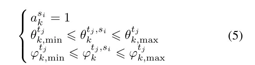
Let akbe the action vector of all ESMs at time step k,wheredenotes the action applied to ESM si(si=1,2,...,NSand NSis the total number of ESM),speci fies whether ESM siis active or inactive at time step k.Considering a limitation of communication bandwidth and processor capacity,only NallESMs can work simultaneously,i.e.,allhave to satisfy the constraint below:

(ii)State space and state transition law

ESMs and targets constitute the main entities of the en-vironment and their states represent the environment states that can be defined aswhereis the state vector of all ESMs,andis the state vector of all targets,With a further unfolding ofand,we yieldandwhich denote the 3-D Cartesian coordinates of the positions and velocities of sensor siand target tj,respectively.Without loss of generality,we define a 3-D coordinate for all ground targets despite the approximate-to-zero height.NTis the number of targets in the surveillance area.

The state transition law is defined by the system dynamic equation sk+1=f(sk,ak,vk),where vkis the process noise.Considering the fact that the activated ESMs will upload their states to the fusion center(agent)at each time step,the agent will pay no attention to their state transition.If we assume that the ground radar targets move independently,then the system dynamic can be decomposed into the state dynamics for each target and since the ESMs work in a passive way,the targets will never know the actions of ESMs,i.e.,the targets’state transition process is independent of the action.

Tsis the sample interval andis the process noise sequence obeying Gaussian distribution with zero mean and covariance.Connect all the targets,the whole system equation can be described as

(iii)Observation set and observation law

The observation law defines how the ESMs originate measurements from the targets or from clutter.The tjth measurement at the sith ESM is given by

When multiple radar targets are present,the measurement equation belonging to ESM siis

(iv)Immediate reward

The primary purpose of adaptive scheduling of multi-ESMs is to maintain a substantial tracking performance of the ground moving radar targets under a limited resource constraint.The posterior Cramer-Rao lower bound(PCRLB)gives a measure of the achievable optimum performance[1],and it represents the average statistical lower bound of estimated tracking error covariance.Letbe an unbiased estimate of system state skat time step k.The PCRLB is defined as the inverse of the Fisher information matrix(FIM):

where Jkis the FIM,and[Jk]-1is the PCRLB.E denotes the expectation over(sk,zk).Jkincludes two parts:the state prior information matrix Js,kand the measurement update information matrix Jz,k:

A recursive formula for the evaluation of the posterior Js,kis given by

where

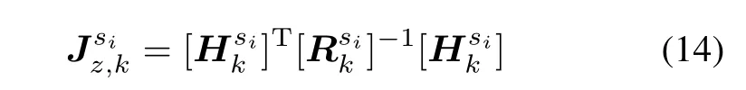
Jz,krepresents the measurement contribution to the FIM.We assume that the ESMs have independent measurement process,then Jz,kcan be written as

Integrating the equations(10)–(15),we will get Jkas

The dimension of Jkis six times larger than the target number,it is extremely intractable for computing the PCRLB that is the inverse of Jk.Hence,here we employ the trace of matrix Jkdirectly as the immediate reward so that the inverse performing process is avoided.

2.3 Agent model

As illustrated in Fig.2,the agent model includes two modules:target tracker and action selector.Target tracker is used for updating the belief state in the uncertain environment with the observations as the inputs.The basic principle of the target tracker module is utilizing Bayesian filter algorithms to update the posterior distribution of the system state.The specific process will be described in Section 3.

The action selector is the decision-making module,which receives the belief state from the target tracker module and selects the optimal policy in a dynamic way.Here,we call it“dynamic”,which means the decision will be made periodically adapting to the dynamic evolution of the environment.To solve this stochastic,dynamic problem,the Markov decision process provides an elegant theory framework,in which the action selector is modelled as to solve the following objective function.

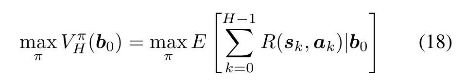
where b0is the initial belief state.is the policy set that is defined as a projection from belief space B to action spaceand.V is the value function that is a projection from belief space B to reward R andrepresents the expected total reward in a time horizon H with an initial belief state b0and an applied policy

Obviously,solving(18)is computationally intractable because it needs to predict and optimize a solution series in a time horizon H.With a little thought,we realize that we do not have to solve this entire problem at once.Suppose we divide the entire time horizon H into M task cycles:[1,l],...,[ml+1,(m+1)l],...,[(M-1)l+1,Ml].Here,l is the sampling frequency of ESM.Then,the agent will make M decisions sequentially instead of one immediate decision and the value function will be re fined as follows:

Equation(19)is the famous Bellman’s equation that converts the original problem into a recursive one.Without loss of generality,for an arbitrary task cycle m(m=1,2,3,...,M),we define Q function:

where r(bml,a)is the expected cumulative reward of current task cycle m andis the expected cumulative reward of future task cycles that begin at time step(m+1)l.

Then for an arbitrary task cycle m,we simply repeat the process of making a decision by solving

Combining the target tracker module and the action selector module,the complete agent model is working as follows:at the beginning of an arbitrary task cycle m,the action selector module figures out the optimal policy according to(22)with belief state bmlas input.Then the selected ESMs will be activated and will continue working till the end of this task cycle.During the working process,ESMs will carry out l samples and the target tracker module will obtain measurements zml+1,zml+2,...,z(m+1)l.Whenever an array of measurements is coming,the belief state is updated by the target tracker module.After l updates,the belief state b(m+1)lwill be available and the m+1 planning begins.

3.Methodology

As discussed in Section1,the recurring challenges in these stochastic,dynamic problems are the partial observability and the curse of dimensionality of the state,especially when dealing with the practical problems.In this section,we present our ADP-based methodology for solving the multi-ESM controlling problem in a ground moving radar targets tracking application.Before a concrete description of the approaches for handling the two challenges referred above,we give a general algorithm framework that can be used to yield optimal policies and schedule ESMs recursively.

Algorithm 1General algorithm framework for online scheduling of multi-ESM

Input:b0the initial belief state

for m=0 to m=M do

for k=ml+1 to k=(m+1)l do

ESMs execute action ak

Collect measurements zkand statesof ESMs

bk←TARGETTRACKER

end for

end for

Algorithm 1 shows the general framework for solving the multi-ESMs adaptive scheduling problem,in which the whole mission is divided into M task cycles.In each cycle,a decision will be made by the action selector,and then the selected ESMs will sample l times in this cycle,and the belief state will be estimated after per sampling by the target tracker.It can be seen that the ACTIONSELECTOR function and TARGETTRACKER function consist the core parts of the algorithm,which will be introduced in detail in the following sections.

3.1 UKF for belief state estimation

As mentioned by Powell[21],if we lack a former model of the information process,even small problems may be hard to solve.Thus the belief state is designed to represent the uncertain and incomplete information and the target tracker module is set to estimate the belief state.The basic idea is to estimate the posterior distribution of the system state using a filtering algorithm.In target tracking application,some filters are maturely used such as KF,EKF,UKF and PF,in which the KF is only applicable to a linear Gaussian system and EKF is an extension of KF that is applicable to a weakly nonlinear Gaussian system.These two methods do have a limited ability to adapt to the problem discussed in this paper.PF and UKF are both appropriate methods that can be applied in any nonlinear system.Despite a wide application in target tracking,PF is essentially a Monte Carlo method facing with the computationally intractability,especially when it is the bottleneck that influences the efficiency of the whole algorithm.For example in Algorithm 1,the filter process is in an inner loop,which means the filtering frequency is exponential with m and l.In this paper,we try to choose the UKF as an instead method for belief state estimating in consideration of trading off the applicability and the computability.

The UKF algorithm approximates a Gaussian stochastic variable using a minimal set of weighted deterministic sample points.In this way,the accuracy of posterior state estimation can hold a second-order Taylor expansion. Con-sidering the deployment principle of ground radar,we assume the multiple radar targets are well separated, and then the belief state can be estimated independently for each target.UKF supposes both the process noise and measurement noise are Gaussian.Under the above assumption,if bk=p(sk|zk)is Gaussian,bk+i=p(sk+i|zk+i)is also Gaussian,and both bkand bk+ican be parameterized by a mean and covariance.Here we give the concrete steps for target tjas follows:

Step 1Sigma produces

Step 2Parameter estimation

Step 3Time update

Step 4Measure update

Step 5State update

Step 6Belief state update

Algorithm 2UKF for belief state estimation

FunctionTARGETTRACKER

Inputs:bk-1,the belief state at time step k-1;zk,the measurements of ESMs at time step k;,the state of ESMs at time step k;

for tj=0 to NTdo

Initialization:Pick up meanand covariancefrom

for i=0 to 2n do

Sigma produce:Caleculateby(23)

Parameter estimation:Calculateby(24);calculateby(25)

Sigma transfer:Calculateby(26);calculateby(29)

end for

Time update:Calculate predict meanby(27)and predict covarianceby(28)

Measure update:Calculate measure updateby(30),(31),(32)

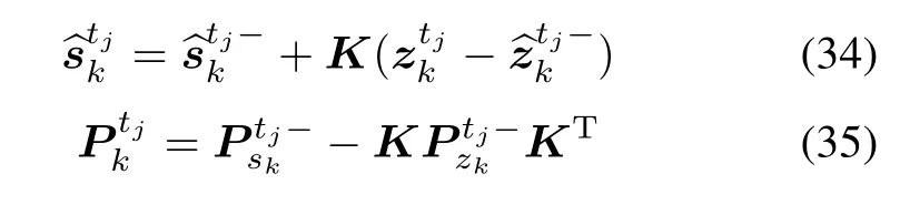
State update:Calculate K by(33)and updateandby(34),(35)

Belief update:Updateby(36)

end for

Outputs:bk

3.2 MCRS for Q-value estimation

According to (22), the precondition of action selecting is to calculate the Q-value under a given belief state and a given action.However,it is hard to carry out a precise calculation of Q for two reasons:one is that the future long-term reward is an optimal value function that needs repeated iterations;the other is that the expectation of reward is non-analytical in the presence of the high-dimensional belief state.In the following section,an approximate approach MCRS will be introduced which combines the advantages of both rollout and Monte Carlo.

3.2.1 Rollout

Rollout is an important technique belongs to approximate dynamic programming.The basic idea of rollout is to design a base policy πband replace the future long-term rewardwithin(20).In this way,the future long-term reward will be approximated in the policy πband will no longer need repeated iterations;namely,(20)will be approximated by

3.2.2 Base policy

Rollout gives the lower bound of the explicit Q-value,which means the base policy πbis particularly important because a better πbwill make the suboptimal policy π∗mmore close to the global optimal policy.

There is no fixed algorithm for base policy designing except a specific treatment for a given problem,such as the closest point of approach(CPA)that is designed to address single target tracking problem[1]and the closest sensors policy(CSP)policy for multiple targets tracking using active sensors[24].In this paper,we focus on the application that multiple ESMs are used to track ground moving radar targets,in which the ESMs are passive,which means they have to be in the electromagnetic radiation region of targets so that they can receive measurements normally.Another characteristic of this application is that the closer the distance between an ESM and a target,the better the tracking performance.Considering the factors above,we designour own base policy and we call it the CCSP to distinguish it from CSP:

3.2.3 Monte Carlo sampling

Another challenge of Q-value estimation is to compute the expectation of the value function in the presence of the high-dimensional belief state.In general,the Monte Carlo method is often used to approximate the expectations of random variables,especially when the distributions of the random variables are accessible.In this paper,we use the belief state to represent the posterior distribution of the system state.Intuitively,we will consider the Monte Carlo method as the key to figure out the dilemma.The specific operating procedure is simple: firstly,we sample N state samplesusing the Monte Carlo method based on the belief state bml;then,for each samplewe compute the cumulative reward of current task cycle in action a and the cumulative reward of the future long-term task cycle in the base policy;Finally,the Q-value will be estimated by averaging over all the samples.

It can be proved that(39)can approximate the Q-value well when the sample size N is large enough.Until now,we have described the Monte Carlo rollout sample approach for the Q-value estimating.Then,we enumerate all the actions,assess the Q-values and select the best policy.Algorithm 3 describes the whole working process of the action selector module.

Algorithm 3MCRS for Q-value estimation and action selection

Function ACTIONSELECTOR(bml)

Input:bml,the belief state at sampling time ml

Base policy:Search the base policyaccordingto(38)

Sampling:Monte Carlo sampling to generate particles

for each action a in A do

for i=1 to N do

Begin calculating current task cycle reward

for k=ml+1 to(m+1)l do

Calculate one-step reward:Ri← Ri+

end for

Finish calculating current task cycle reward

Begin calculating future task cycle long-term reward

for m=m+1 to M-1 do

Calculate one-step reward:Vi←Vi+

end for

end for

Finish calculating future task cycle long-term reward

Calculate total pro fit:Q←Q+Ri+Vi

end for

Calculate average reward:Q←Q/N

if Q＞maxQ do

maxQ←Q

end if

end for

4.Numerical experiments

4.1 Experiments set-up

In this section,we consider an application that several UAVs are placed in the airspace to detect and track a set of ground moving radar targets.Each UAV carries an ESM sensor on-board that can track radar targets by detecting the electromagnetic radiation of the radar passively.Consider an eight UAVs(S1–S8)versus four radars(T1–T4)scenario,so we get NS=9 and NT=4.Assuming the initial locations of the UAVs are{S1(3,6,3),S2(6,6,3),S3(9,6,3),S4(3,6,6),S5(6,6,6),S6(9,6,6),S7(3,6,9),S8(6,6,9),S9(9,6,9)}(km,km,km),which are defined in the Cartesian coordinate system with(x,y,z)indicating(north,sky,east).All the UAVs are in a circular motion with a constant velocity100m/s.The ESM on-board has a frequency band from 0.5 GHz to 40 GHz that can cover the targets’ radar frequency and all the ESMs are assumed owning the same azimuth measurement accuracyand the same pitch measurement accuracywhich determines the measurement covariance matrixThe sampling interval is set up to Ts=4 s.Considering the resource limitation of communication and computation,there are only Nall=4 ESMs allowed to work at the same time.

4.2 Tracking performance

To demonstrate the performance of the policy deriving from our MCRS approach,we pick up three other commonly used policies,which are the myopic policy,the CCSP policy and the random policy.As comparisons,the myopic policy ignores the future long-term reward and makes decision only by maximizing the immediate reward Rk;the CCSP policy is the base policy designed in this paper and the policy is figured out based on(38);Random policy means to select a policy randomly at every decision point.Within the 100 s time horizon,there are ten planning processes,and the action sequences are illustrated in Fig.3,where Fig.3(a),Fig.3(b),Fig.3(c),Fig.3(d)are the myopic policy sequences,the CCSP policy sequences,the random policy sequences,and the MCRS policy sequences,respectively.

At every decision point,the agent should select four ESMs from the total eight ESMs to track the four ground moving radar targets.As depicted in Fig.3,the horizontal axis is the time steps,while the vertical axis represents the number of the candidate ESMs.Whenever a symbol“*”is marked in a vertical axis scale,it means the corresponding ESMs are selected in this cycle.For instance,consider the Fig.3(d)of the MCRS policy,we can figure out the result that the ESMs(S2,S3,S4,S7)are selected in the first cycle(0–20 s),which means the action isBy that analogy,we can derive all the actions of the next nine task cycles are a2=[1,1,0,1,1,0,0,0,0]T,a3=[0,1,0,0,1,0,1,1,0]T,a4= [0,1,0,0,1,0,1,0,1]T,a5=[0,1,1,0,1,1,0,0,0]T,a6=[0,0,1,0,1,1,0,0,1]T,a7=[0,0,1,0,1,1,0,0,1]T,a8=[0,0,1,1,0,0,1,0,1]T,a9=[0,1,1,1,0,0,0,0,1]T,a10=[0,0,0,1,0,1,1,0,1]T,respectively.

Fig.3 Action sequences of the four typical policies

Then,we can give the action sequences of all the four typical policies by matrix.

Fig.4 compares the cumulative rewards of the four typical policies in the ten planning processes.Obviously,the MCRS policy provides a bigger cumulative reward than the myopic policy,the CCSP policy and the random policy.It is not surprising that the MCRS policy outperforms another three policies because not only does the MCRS policy considers a long-term reward in decision-making,but also it carries out an policy improvement process comparing to CCSP.Also,we have a fact that cumulative rewards of the myopic policy is remarkably smaller than the CCSP policy,the random policy and the MCRS policy,since the latters all belong to non-myopic politics that take a long-term reward into account when making a decision.To compare in the horizontal direction,we will find a law that the cumulative rewards decrease progressively.The main reason for this is that as time processes,the future time horizon will get smaller and smaller for a finite horizon problem,and the future long-term reward will be smaller and smaller.

Fig.4 Comparison of cumulative rewards of the four typical policies

To have further analysis of the efficiency of the four typical politics,we compare the tracking performance of our MCRS policy to the rest three ones.As illustrated in Fig.5,we select the position root-mean-square(RMS)error as the indicator and Fig.5(a),Fig.5(b),Fig.5(c),Fig.5(d)provide the tracking performance comparing of target T1,T2,T3 and T4,specifically.Again,we draw a conclusion that the MCRS provides a smaller average position RMS error than another three politics,and the superiority will be more and more obvious as time goes on,which demonstrate the tracking stability of the MCRS policy.

5.Conclusions and future work

In this paper,we investigate the adaptive controlling for multi-ESMs to track the ground moving radar targets.Since the environment is uncertain and dynamic,we adopt the dynamic programming theory to describe the problem with an environment model and an agent model.With the consideration of a long-term cumulative reward when choosing current sensing actions,the ADP framework provides a better performance than some general programming models.Then,to solve the computationally intractable ADP problem,we address the challenges of the partial observability and the curse of dimensionality with two related modules and approaches.The UKF algorithm is adopted to approximately estimate the belief state that provides a basis for the decision-making,and an MCRS algorithm is proposed for estimating the Q-value with a combination of the rollout method and the Monte Carlo method that belongs to ADP algorithms.A heuristic base policy CCSP is proposed for approximating the future long-term cumulative rewards.The experiments on a multi-ESMs controlling problem including eight ESMs for tracking four separated ground moving radar targets demonstrate the effectiveness of the proposed approach.

Notice that the technique proposed in this paper outperforms other strategies in a larger-scale problem,but the scale of the sensor network is still limited.When the sensor amount increases,the action space will grow exponentially.Then,the curse of dimensionality with respect to action space will become a big challenge when the agent carries out the action selecting process.A heuristic action generating algorithm or some intelligent action sampling methods will be designed in our future work in a bid to alleviate a larger-scale problem than this paper.Furthermore,a varying number of targets will be considered to replace the fixed number of targets assumption in this paper.

Acknowledgment

I would like to thank the Key Laboratory of Aerospace Information Perception and Photoelectric Control Ministry of Education,which provides me a good research platform and study environment.I also thank my fellow graduate students for their help and support, especially Junfeng Mei,who help to correct many written mistakes.

[1]HE Y,CHONG E K P.Sensor scheduling for target tracking:a Monte Carlo sampling approach.Digital Signal Processing,2006,16(5):533–545.

[2]SCOTT A M,ZACHARY A H,CHONG E K P.A POMDP framework for coordinated guidance of autonomous UAVs for multitarget tracking.EURASIP Journal on Advances in Signal Processing,2009,2009(1):1–17.

[3]YAOP,WANGH,SUZ.Real-time path planning of unmanned aerial vehicle for target tracking and obstacle avoidance in complex dynamic environment.Aerospace Science&Technology,2015,47:269–279.

[4]SHAFERMAN V,SHIMA T.Tracking multiple ground targets in urban environment using cooperating unmanned aerial vehicles.Journal of Dynamic Systems Management&Control,2015,137(5):1–11.

[5]ZHANG M,LIU H.Cooperative tracking a moving target using multiple fixed-wing UAVs.Journal of Intelligent&Robotic System,2016,81(3):505–529.

[6]HERNANDEZ M L,KIRUBARAJAN T,BAR-SHALOM Y.Multisensor resource deployment using posterior Cramer-Rao bounds.IEEE Trans.on Aerospace and Electronic Systems,2004,40(2):399–416.

[7]LI B B,KIUREGHIAN A D.Robust optimal sensor placement for operational model analysis based on maximum expected unity.Mechanical System and Signal Processing,2016,75:155–175.

[8]GONG X,ZHANG J,COCHRAN D.Optimal placement for barrier coverage in bistatic radar sensor networks.IEEE/ACM Trans.on Networking,2016,24(1):259–271.

[9]LIU X,SHAN G,SHI J.Multi-sensor allocation based on Cramer-Rao low bound.Proc.of IEEE Workshop on Electronics,Computer and Applications,2014:467–470.

[10]VERMA A,AKELLA M,FREEZE J.Sensor resource management for sub-orbital multi-target tracking and discrimination.Proc.of AIAA Space Flight Mechanics Meeting,2015:1647–1662.

[11]GOSTAR A K,HOSEINNEZHAD R,BAB-HADIASHAR A.Robust multi-Bernoulli sensor selection for multi-target tracking in sensor networks.IEEE Signal Processing Letters,2014,20(12):1167–1170.

[12]ZOGHI M,KAHAEI M H.Adaptive sensor selection in wireless sensor networks for target tracking.IET Signal Processing,2010,4(5):530–536.

[13]BEJAR R,KRISHNAMACHARI B,GOMES C.Distributed constraint satisfaction in a wireless sensor tracking system.Proc.of the Workshop on Distributed Constraint Reasoning,2001:81–90.

[14]HORRIDGE P R,HERNANDEZ M L.Performance bounds for angle-only filtering with application to sensor network management.Proc.of the 6th International Conference on Information Fusion,2003:695–703.

[15]HAUNG C F.The coverage problem in a wireless sensor network.Proc.of the 2nd ACM International Conference on Wireless Sensor Networks and Applications,2003:115–121.

[16]GUPTA V,CHUNG T H.On a stochastic selection algorithm with applications in sensor scheduling and sensor coverage.Automatica,2006,42(2):251–260.

[17]THARMARASA R.Sensor management for large-scale multisensor-multitarget tracking.Hamilton,Canada:McMaster University,2007.

[18]RISTIC B,VO B N,CLARK D.A note on the reward function for RHD filter with sensor control.IEEE Trans.on Aerospace&Electronic Systems,2011,47(2):1521–1529.

[19]HOANG H G.Control of a mobile sensor for multi-target tracking using multi-target/object multi-Bernoulli filter.Proc.of International Conference on Control,Automation and Information Sciences,2012:7-12.

[20]DARIN C H.Stochastic control approaches for sensor management in search and exploitation.Massachusetts,USA:Boston University,2010.

[21]WARREN B P.Approximate dynamic programming:solving the curses of dimensionality.New Jersey:Wiley Press,2010.

[22]CHRIS K,DORON B,ALFRED H.Adaptive multi-modality sensor scheduling for detection and tracking of smart targets.Digital Signal Processing,2006,16(5):546–567.

[23]BAR-SHALOM Y,LI X,KIRUBARAJAN T.Estimation with applications to tracking and navigation.New Jersey:Wiley Press,2011.

[24]LI Y,KRAKOW L W.Approximate stochastic dynamic programming for sensor scheduling to track multiple targets.Digital Signal Processing,2009,19(6):978–989.

[25]BERTSEKAS D P,TSITSIKLIS J N.Neuro-dynamic programming.Massachusetts:Athena Scientific Press,1996.

[26]SHAWE-TAYLOR J,CRISTIANINI N.Kernel methods for pattern analysis.Journal of the American Statistical Association,2006,101(476):1730.