Idealized Experiments for Optimizing Model Parameters Using a 4D-Variational Method in an Intermediate Coupled Model of ENSO
2018-03-06ChuanGAORongHuaZHANGXinrongWUandJichangSUNKeyLaboratoryofOceanCirculationandWavesInstituteofOceanologyChineseAcademyofSciencesQingdao26607China
Chuan GAO,Rong-Hua ZHANG,Xinrong WU,and Jichang SUNKey Laboratory of Ocean Circulation and Waves,Institute of Oceanology,Chinese Academy of Sciences,Qingdao 26607,China
2Qingdao National Laboratory for Marine Science and Technology,Qingdao 266237,China
3Institute of Oceanographic Instrumentation,Shandong Academy of Sciences,Qingdao 266001,China
4University of Chinese Academy of Sciences,Beijing 100029,China
5Key Laboratory of Marine Environmental Information Technology,State Oceanic Administration,National Marine Data and Information Service,Tianjin 300000,China
1.Introduction
The El Niño–Southern Oscillation(ENSO)is the strongest interannual signal of the climate system(Bjerknes,1966),which has significant impacts on the weather and climate worldwide through atmospheric teleconnection(e.g.,Huang et al.,2001;Xie et al.,2010).At present,the ENSO phenomenon is recognized as comprising of the most predictable short-term climate anomalies thanks to successful development of air–sea coupled models(e.g.,Chen et al.,2004;Zhang et al.,2013),including intermediate coupled models(ICMs;e.g.,Zebiak and Cane,1987;Zhang et al.,2003).Currently,various coupled models enable us to make six-month and longer real-time ENSO predictions in advance with reasonable success.For example,we developed an improved ICM at the Institute of Oceanology, Chinese Academy of Sciences(IOCAS),named the IOCAS ICM(Zhang and Gao,2016a).The model has been routinely used to predict SST evolution in the tropical Pacific(for a summary of the model’s ENSO forecasts,see the International Research Institute for Climate and Society website at http://iri.columbia.edu/climate/ENSO/currentinfo/update.html). Nevertheless,IOCAS ICM still has systematic biases with large uncertainties in ENSO prediction(Zhang and Gao,2016b).
Various methods have been developed to improve the quality of ENSO forecasts,which are affected by many factors,including the model itself and the initial conditions that are used to make predictions (Mu et al.,2002).To improve the ENSO prediction skill,one effective way is to calibrate the model prediction of ENSO by designing model-dependent statistical correction methods(Ren et al.,2014;Liu and Ren,2017).Also,one of the sources for ENSO prediction errors is the initial ocean conditions,because the initial error can grow and amplify through ocean dynamics and air–sea interactions.As observations are still sparse in the ocean,limited observational data need to be combined with models in a smart way to provide coherent initial conditions that are consistent with model dynamics(Wang et al.,2000).Recently,data assimilation methods have been successfully used to optimize the initial conditions for ocean model initialization,which can significantly improve ENSO simulation and prediction.Various data assimilation methods are currently available,including the Ensemble Kalman Filter(EnKF)and variational data assimilation methods(Dommenget and Stammer,2004;Zhang et al.,2005b;Zheng et al.,2006,2009;Wu et al.,2016).
Another major source for ENSO prediction errors comes from model errors,including uncertainties in model parameters(Mu et al.,2010).Physically,model parameters are introduced to represent processes and quantify the relationships between related fields.Inevitably,approximations are often made in estimating parameters to represent real physics.Observations can be used to tune model parameters in a simple and straightforward way(Wu et al.,2012).Often,parameters are estimated in an empirical and subjective way,and such an a priori estimate of parameters may not be consistent with model dynamics.It is desirable to estimate parameters in an optimal way,in the sense that the best possible simulations can be produced for a given model(Liu et al.,2014).Furthermore,model error characteristics could be taken into account,and it is thus preferable to be able to automatically consider the feedback of model dynamics to parameter estimates.The 4D variational(4D-Var)data assimilation approach offers such an objective and comprehensive way to optimize model parameters for improving model simulations.Indeed,the variational data assimilation method has been widely applied to parameter estimation in ocean models.For example,Lu and Hsieh(1998)implemented an adjoint assimilation method into a simple equatorial air–sea coupled model to investigate the optimization of initial conditions and model parameters.Zhang et al.(2005b)examined the ability of the 4D-Var method to optimize the uncertainty of model parameters.Peng and Xie(2006)and Peng et al.(2013)developed a 4D-Var algorithm to correct the initial condition and wind stress drag coefficient for storm surge forecasting.Zhang et al.(2015)assimilated SST data in a two-equation turbulence model by 4D-Var data assimilation to estimate the wave-affected parameters.These studies clearly indicate that the combination of optimizing initial conditions and optimizing model parameters through data assimilation can effectively improve model simulation and prediction.
In this study,we continue to channel our efforts into improving IOCAS ICM for better ENSO simulation and prediction.One way to improve its performance is through data assimilation.To this end,a 4D-Var data assimilation method has been implemented into the ICM to improve state analyses(Gao et al.,2016),which provides an optimal initial state that can be used to predict ENSO.However,this previous study only applied data assimilation to optimizing the ocean initial state.Because severe biases can be apparently derived from errors in model parameters,it is desirable to use the 4D-Var scheme and develop a method to optimize model parameters in combination with optimizing initial conditions.
Here,we aim to implement a framework for optimizing model parameters in the ICM through the 4D-Var data assimilation system,and demonstrate the feasibility of constraining ENSO evolution.As described before(Zhang and Gao,2016a),one important feature of IOCAS ICM is the way in which the temperature of the subsurface water entrained into the mixed layer(Te)is parameterized;the thermocline effect on SST in the ICM is explicitly represented by the relationship between Teand sea level(SL;an indicator of thermocline fluctuation),written as Te=αTeFTe(SL),in which SL represents the thermocline variability,FTeis the relationship between the Teanomaly and SL anomaly derived using empirical statistical methods(such as SVD),and αTeis a scalar parameter introduced to represent the intensity of subsurface thermal forcing.Various studies have found that subsurface thermal effects(such as entrainment and mixing)play an important role in ENSO evolution(Ballester et al.,2016;Zhang and Gao,2016a).Indeed,our previous studies have shown that ENSO simulations are very sensitive to αTe(e.g.,Gao and Zhang,2017).Here,this parameter is chosen to demonstrate a way in which optimal parameter estimation can be achieved using the 4D-Var method equipped within the ICM.The effects of optimizing this parameter on the simulation and prediction of ENSO are examined,with the feasibility of the approach in recovering the ENSO evolution demonstrated.
The paper is organized as follows:Section 2 describes the ICM,the parameter estimation procedure using the 4D-Var data assimilation method,and the experimental setup.The effects of the parameter estimation on the simulation and prediction of ENSO are analyzed in sections 3 and 4,respectively.Finally,a conclusion and discussion are presented in section 5.
2.Methodology
In this paper,we examine the feasibility and effectiveness of optimizing a model parameter in improving ENSO simulation and prediction using the 4D-Var data assimilation method implemented in the ICM.In this section,we briefly introduce the methodology used to optimize the model parameter based on the 4D-Var method.First,a short description of the ICM is presented.Second,the 4D-Var data assimilation scheme and optimal parameter estimation method are introduced.Finally,results from a twin experiment are used to demonstrate the feasibility of the approach,and the effects of optimal initialization and parameter estimation on ENSO evolution are compared.
2.1.Description of the ICM
The ICM used is an anomaly model consisting of an intermediate ocean model(IOM)and an empirical wind stress model(Fig.1).One crucial aspect of the ocean component is the way in which the subsurface entrainment temperature in the surface mixed layer(Te)is explicitly parameterized in terms of the thermocline variability(as represented by the SL),written as Te=αTeFTe(SL),in which FTeis the relationship between the anomalies of Teand SL derived using statistical methods from historical data.A parameter,αTe,is introduced in the ICM to represent the intensity of thermal forcing associated with subsurface anomalies(Zhang et al.,2005a).
The model has already been successfully used for ENSO simulations and predictions;see Zhang and Gao(2016a)for more details. Various model parameters exist within the ICM;here,we pay special attention to the parameter αTe,since it represents the intensity of the thermocline feedback,an important parameter to ENSO.
2.2.Optimal parameter estimation based on the 4D-Var data assimilation system
Previously,we successfully implemented the 4D-Var method into the ICM and demonstrated that optimal initialization of the ocean state can improve ENSO simulation and prediction skill(Gao et al.,2016).However,the importance of variational estimation for major model parameters to ENSO in the ICM has not been demonstrated.Here,we aim to develop a modeling framework for optimizing model parameters using the 4D-Var method,which can be used further for improving real-time ENSO prediction.
Variational methods(3D-Var and 4D-Var),as a sophisticated branch of data assimilation,convert the problem of seeking the optimal initial state to that of minimizing a cost function under the constraint of model dynamics.More specifically,optimal control theories are applied to ocean–atmosphere models,which act as a constraint in the minimization of the cost function representing the mis fi ts between model simulation and observation(Courtier et al.,1994).For example,the 4D-Var data assimilation method utilizes observational data within a data insertion time window,seeking optimal values of model variables and parameters by minimizing the cost function under dynamical constraint.As the control variables are adjusted,the mis fi ts are reduced accordingly between the model solution and observation.
Generally,an adjoint model is an efficient solution for evaluating the gradient of the cost function with respect to high-dimensional control variables in the 4D-Var data assimilation method.The adjoint model of the ICM is written coding-by-coding.First,the tangent linear model of the ICM is obtained by linearization.Then,the adjoint model of the ICM is achieved by transposing the tangent linear model;i.e.,it features the reverse of the temporal and spatial integration and other characteristics.In fact,the tangent linear model does not directly participate in the 4D-Var assimilation system.It is only used to validate the correctness of the adjoint model of the ICM.More details can be seen in Gao et al.(2016).
Optimal parameter estimation is realized through the 4DVar assimilation of observational data under the constraint of model dynamics.Previously,a 4D-Var data assimilation system has already been successfully constructed in the ICM(Gao et al.,2016);model parameters can then be optimized.specifically,the governing equations of the ICM can be expressed as follows(Kalnay,2003):

where t is time and t0is the initial time;is the vector of control variables in the ICM;represents the model parameters to be optimized,in which q is the total number;is the initial value ofis the initial value ofand F is the nonlinear forward operator.
For the parameter estimation in the 4D-Var data assimilation context,the cost function can be formulated as(Kalnay,2003)
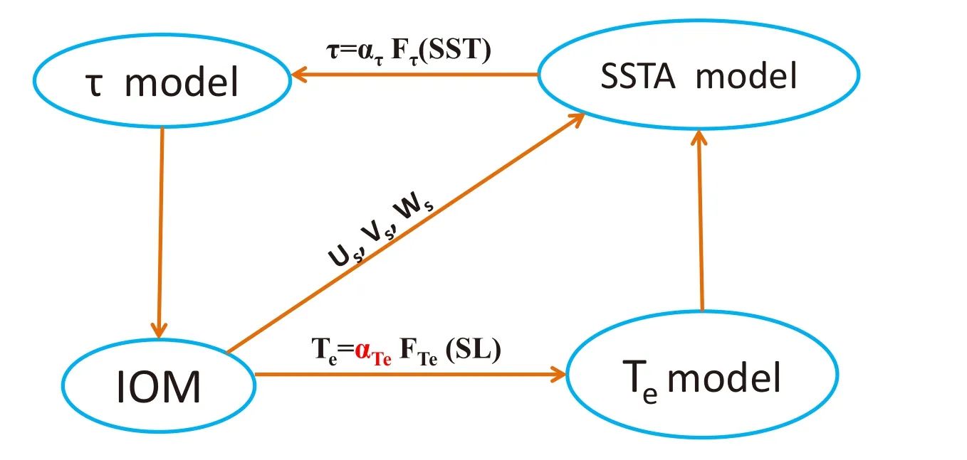
Fig.1.Schematic diagram showing the components of IOCAS ICM,consisting of an IOM and various anomaly models for wind stress(τ),SST and Te.See the main text for more details.
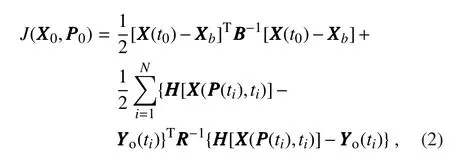
where the first term on the right-hand side is the background error term and the second is the observation error term.The superscript“T”represents the transpose of a matrix and the subscripts“b”and“o”represent the background field and observation,respectively;N indicates the number of integrations in the minimization time window;represents the observation;andrepresent the background error covariance matrix,the observation error covariance matrix and the observation operator,respectively.In this study,andand are simply set as diagonal matrices,which are the identity matrix multiplied by the standard deviation of the observation.The parametersare implicitly expressed in the cost function,which are regarded as independent variables ofand the gradient of the cost function with respect toandis calculated by the adjoint model of the ICM.Essentially,the process of parameter estimation based on the 4D-Var method is the same as the optimal initialization process for obtaining the initial conditions,which is detailed in Gao et al.(2016).
Figure 2 illustrates the procedure involved with the 4DVar algorithm in obtaining the optimized initial condition and parameters in the ICM.The Specific steps are as follows:First,for a given initial guess(model solution),model parameterand observationthe ICM is integrated forward to obtain the cost function J(a mis fi t between the model solution and observation).Second,the ICM is integrated backward with the adjoint model to obtain the gradient of J with respect toandandThird,a minimization process is performed to obtain optimal analysis solutions of the initial condition and model parameters;here,the Limited-Memory Broyden–Fletcher–Glodfarb–Shanno(L-BFGS)algorithm(Liu and Nocedal,1989)is adopted to minimize the cost function to reduce the mis fi t and obtain the optimal analysis field.When the gradient calculation converges to a value that satis fi es a certain level of precision,the iteration is stopped and an optimalfield andvalue are obtained;otherwise,the resultantandare used as a new estimate and the steps outline above are repeated.
2.3.Experimental setup
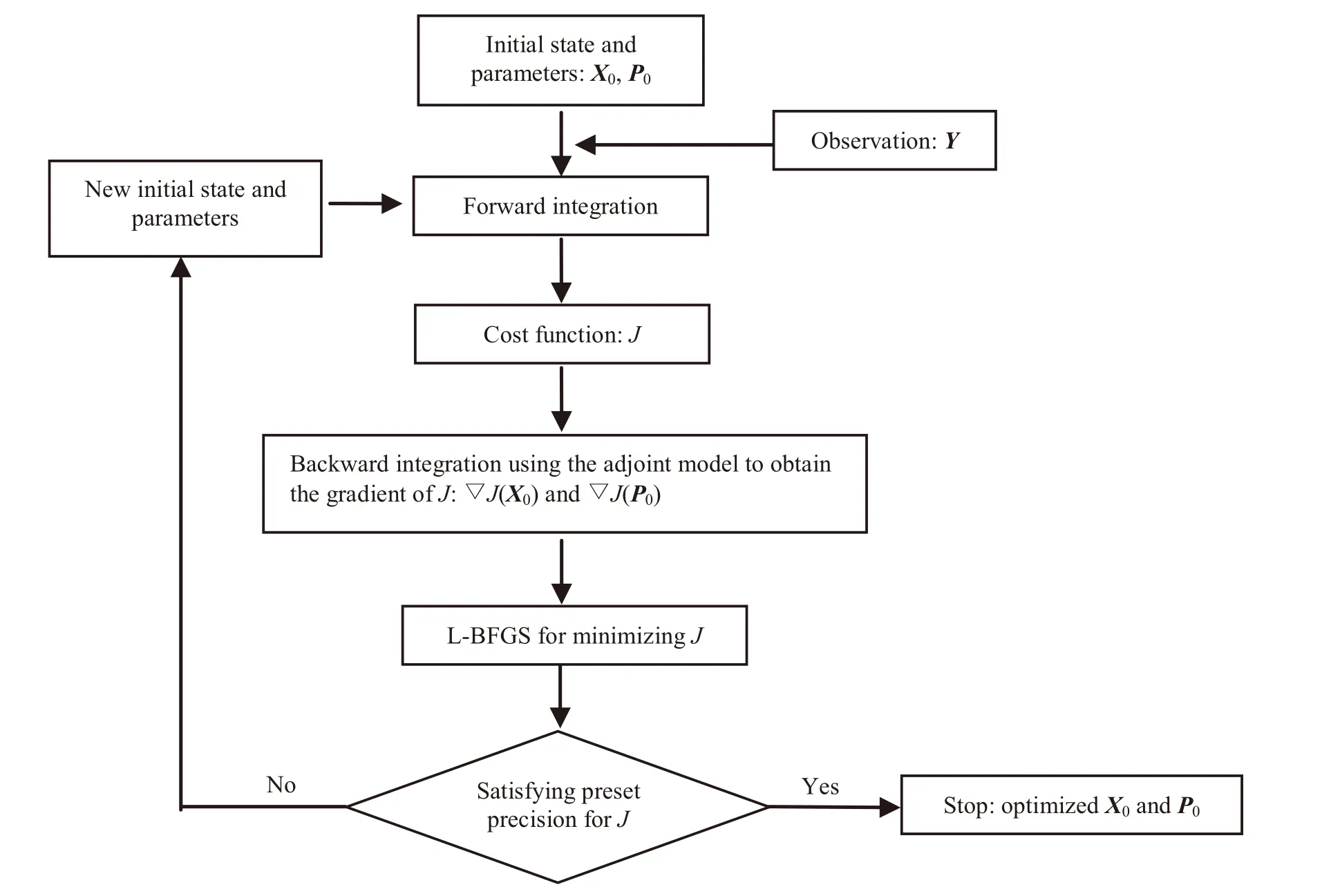
Fig.2.Schematic diagram illustrating the procedure to optimize the ocean initial state)and model parametersusing the 4D-Var data assimilation system.
Our previous studies have shown that initial conditions can be optimized in the ICM through the 4D-Var assimilation of SST data to effectively improve ENSO simulation and prediction(Gao et al.,2016).Based on this,in this paper,a new application is demonstrated using the ICM-based 4DVar system for optimal parameter estimation.As mentioned above,αTeis an empirically introduced scalar parameter representing the intensity of the subsurface thermal effect on SST,which has an important influence on ENSO evolution.Thus,as an example,αTeis chosen to demonstrate the feasibility and effectiveness of the 4D-Var-based optimization of parameter estimation in improving ENSO modeling.
A twin-experiment strategy is adopted.Two basic experiments are performed first.A control run is conducted using the ICM with its standard parameters,including the coupling coefficient between interannual anomalies of SST and wind stress(τ), ατ=1.03;vertical diffusivity coefficient,Kv=1.0×10⁻³;thermal damping coefficient for SST anomalies,λ=1/(100×86400);and the coefficient between anomalies of Teand SL,αTe=1.0.As shown in Gao et al.(2016),the control run simulates ENSO very well.A “biased”run is then conducted,in which some modifications are made to these model parameters,as follows:ατ=1.03×1.01;Kv=1.0×10−3×0.95;λ =1/(100×86400)×1.01;and αTe=1.1.Here,the ICM with these modified parameters is referred to as the “biased”model,considering a situation in which model errors are erroneously produced by the changes in these model parameters.Here,the changes in these parameters(ατ,Kv,λ)are quite subtle,to guarantee the periodic oscillation of ENSO.If the changes in the parameters are excessive,it may break the balance of the dynamical processes,and the oscillation will not be maintained.Note that αTeis set to have its change a little bigger for testing how well the parameter optimization using the 4D-Var method will work.
Next,we examine the extent to which the ENSO evolution simulated using the “biased”model can be recovered through the 4D-Var assimilation of the SST data,which are taken from the control run.We refer to the control run as Expt.1,which is integrated for 20 years using the “truth”model(with the default model parameters and “truth”initial condition)to generate the “truth”or “observed”data.The daily“observed”SST field is sampled from the“truth”model simulation with a Gaussian noise added to mimic the“observation”error.The mean and standard deviation of“observational”SST error are set to be zero and 0.2°C.The constructed “observation”of SST data from Expt.1 is used for assimilation into the “biased”model.Note that the type of observational error approximated in this way is rather simple,and it is not the basic question to be focused on here;instead,a key focus is to demonstrate the effectiveness of parameter optimization using the 4D-Var method.
Based on these basic runs,two optimizing experiments using the “biased”model are designed as follows(Table 1):Expt.2 uses the “biased”model in which the initial conditions are optimized by assimilation of the “observed”SST data from Expt.1.Expt.3 is a combined optimizing experiment,in which the initial condition and model parameter(αTe)are simultaneously optimized through assimilating the“observed”SST data from Expt.1.Notethatdaily“observed”SST data are assimilated into the “biased”model in Expt.2 and Expt.3 only at the first time-step of every month.The length of the assimilation window is set to be one month in consideration of the computational efficiency.The period of the experiments is 20 years,from model time 2060/01/01 to 2079/12/31.Comparisons of the ENSO evolution between these experiments(Expt.1,Expt.2 and Expt.3)are made to show how the optimization works and its effect on the recovery of ENSO features.Furthermore,a series of oneyear hindcast experiments are performed using the “biased”model,in which the optimized analyses(initial state and/or model parameter)are taken on the first day of each month when making hindcasts;the hindcast periods are from model time 2062/01/01 to 2079/12/01 after a 2-year spin-up period in the optimizing experiments.
3.Effect on ENSO simulation
The main purpose is to see how ENSO evolution in the“biased”model can be recovered using the 4D-Var assimilation of“observed”SST data sampled from the truth model.To this end,in this section,we examine how well the parameter αTeis optimized,which can lead to a recovery of ENSO evolution.Also,we compare the effects on ENSO simulations between experiments having only the initial condition optimized,and having both the initial condition plus this additional model parameter optimized.Based on these results,an effective way to recover the ENSO evolution is demonstrated through additionally optimizing this model parameter.
3.1.Optimized estimate of the model parameter
The “truth”value of αTeis 1.0 in the control experiment(Expt.1),and αTeis erroneously set to a “biased”value of 1.1 in Expt.2 and Expt.3 when using the “biased”model.The optimizing experiments are designed to see whether the“truth”αTevalue(1.0)can be recovered from the “biased”αTevalue in the “biased”model by the optimizing procedure using the 4D-Var assimilation of SST data taken from the “truth”model.Figure 3 shows the time series of αTeestimated from the first eight-year assimilation in Expt.3.It is seen that the estimated αTetends to approach the “truth”value through the optimization,which keeps a steady state after the first two-year spin-up period.In particular,the rescaled view shown for clarity in Fig.3 indicates that,after a few years of optimization,the optimized αTeduring the fiveto eight-year simulation in Expt.3 is in a steady state,being approximately 1.0.These results indicate that the model parameter can be effectively and reasonably well optimized by the 4D-Var-based method.The parameter estimation procedure is feasible and can give rise to the expected value.

Table 1.Twin-experiment design using 4D-Var-based assimilation of SST data.Expt.1 is a control experiment using the“truth”model,in which the“observation”of SST data is obtained.Expt.2 is an optimizing experiment using a“biased”model,in which the initial condition is optimized through assimilation of“observed”SST data obtained from Expt.1.Expt.3 is a combined optimizing experiment using the “biased”model,in which the initial condition and model parameter are both optimized through assimilation of“observed”SST data obtained from Expt.1.
3.2.Recovery of ENSO evolution
In this subsection,we examine the evolution of various anomaly fields.As described above,the “biased”model is used to perform the optimizing experiments,with assimilation of SST data for only the initial condition in Expt.2,and the initial condition plus the model parameter in Expt.3,respectively.Figure 4 shows the longitude–time sections of SST anomalies along the equator from the simulations in Expt.1,Expt.2 and Expt.3 during the first 12-year simulation.The similarity indicates the effectiveness of the recovery.It is clearly illustrated that simulations based on Expt.2 and Expt.3 can both recover the basic characters of ENSO events well,including the period,spatial distribution,phase transition,and so on.For instance,after approximately the first two-year spin-up simulation period,the SST simulated in Expt.2(Fig.4b)is recovered to its“truth” field(Fig.4a)when the “observed”SST data are assimilated into the “biased”model.However,because of model parameter error,several departures still exist compared with the “truth” field.For example,the amplitude of the SST anomaly in Expt.2 is much larger than the“truth” field,and the phase transition time is changed slightly.By contrast,the SST field in Expt.3(Fig.4c)can recover to the “truth” field quickly(Fig.4a)after a short spin-up period.Thus,comparing these three experiments clearly indicates that additionally optimizing this model parameter using the 4D-Var assimilation of SST data can further improve ENSO simulation.
It is expected that optimizing the model parameter αTecan have a direct influence on the Tefield when assimilating the “observed”SST data.Figure 5 shows the longitude–time sections of Teanomalies along the equator for the “truth”field,Expt.2 and Expt.3,during the first 12-year simulations.For Expt.2(Fig.5b),in which the model parameter αTeis not optimized,the Tefield can be seen to recover through assimilating the“observed”SST data.However,several departures still exist compared with the “truth” field(Fig.5a),which are induced by model parameter biases.It can be seen that a larger αTe(αTe=1.1)acts to produce a simulated Tefield that is also larger—consistent with our previous studies indicating that the subsurface thermal effect is stronger when αTeis chosen to be larger(Zhang and Gao,2016a).Therefore,when the subsurface effect on SST is stronger,the SST simulated in Expt.2 is larger than that of the “truth” field(Fig.4b).However,when αTeis optimized in Expt.3 to the “truth”model parameter(αTe=1.0;Fig.3)by parameter estimation based on assimilating the“observed”SST data,the simulated Teof Expt.3(Fig.5c)closely resembles the“truth” field.All these results indicate that optimizing both model parameters and the initial state through 4D-Var-based SST assimilation can recover the ENSO evolution more effectively than just optimizing the initial state alone.
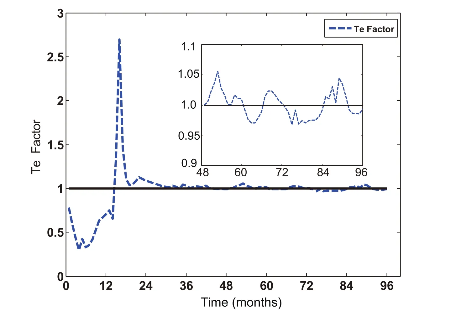
Fig.3.Time series of αTeestimated optimally using the 4D-Var method during the first eight-year assimilation periods.For clarity,a rescaled(ampli fi ed)view is also embedded in the figure for the αTeestimated during the five-to eight-year assimilation periods.
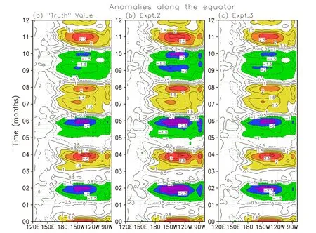
Fig.4.Longitude–time sections of SST anomalies along the equator for(a)the “truth” field,(b)Expt.2 and(c)Expt.3 during the first 12-year simulation period.The contour interval is 0.5°C.
3.3.Quanti fi cation in terms of the RMSE
To quantify the effect on ENSO simulation of parameter estimation optimization,the RMSEs for some major variables are calculated.Here,the RMSE is defined as follows:

Figure6 shows the RMSE time series for the anomalies of SST,wind stress,SL and Tecalculated over the full model domain(30°N–30°S,124°E–78°W).Expt.2 is a case in which only the initial condition is optimized by assimilating SST data;whereas,in Expt.3,both the initial condition and the model parameter are optimized.The results shown in the lefth and panels are calculated on the first day of each month in the first two-year simulation,and those in the right-hand panels are for the 3–12-year simulation for Expt.2(blue)and Expt.3(red).It is clearly evident that the RMSEs of both experiments decline consistently and systematically,reaching a steady state.Nevertheless,compared to Expt.2 without parameter estimation,the RMSEs of Expt.3 decline faster,being more effective at reaching the steady state(left-hand panels in Fig.6).Additionally,the values of the RMSEs are much smaller in Expt.3 compared with those in Expt.2 when reaching the steady state(right-hand panels in Fig.6).As with previous research in which it was shown that optimal initialization based on the 4D-Var method can effectively reduce the RMSEs of some major variables for ENSO simulation(Gao et al.,2016),here,optimal initialization and parameter estimation combined,based on4D-VarSST assimilation,work well too.Furthermore,it is also illustrated that parameter estimation based on assimilating SST data using the 4D-Var method can further improve the recovery of the simulation of the “truth” field using the “biased”model.Thus,ENSO simulations can be improved by simultaneously optimizing the initial conditions and model parameters through the 4D-Var assimilation of SST data.
Next,the spatial distributions of the RMSEs are examined for some major model variables.Here,the RMSEs for each grid are calculated as follows:
(2)地表水。井田南西侧有下山河,在临近河谷地带开采,采空区可引起地表开裂与塌陷,从而沟通地表水体,导致地表水溃入井巷。在其附近地段开采时,应加强顶板管理以及注意地表水体周边隐伏断层沟通地表水,以防水害发生。


Fig.5.As in Fig.4 but for Teanomalies.The contour interval is 1°C.
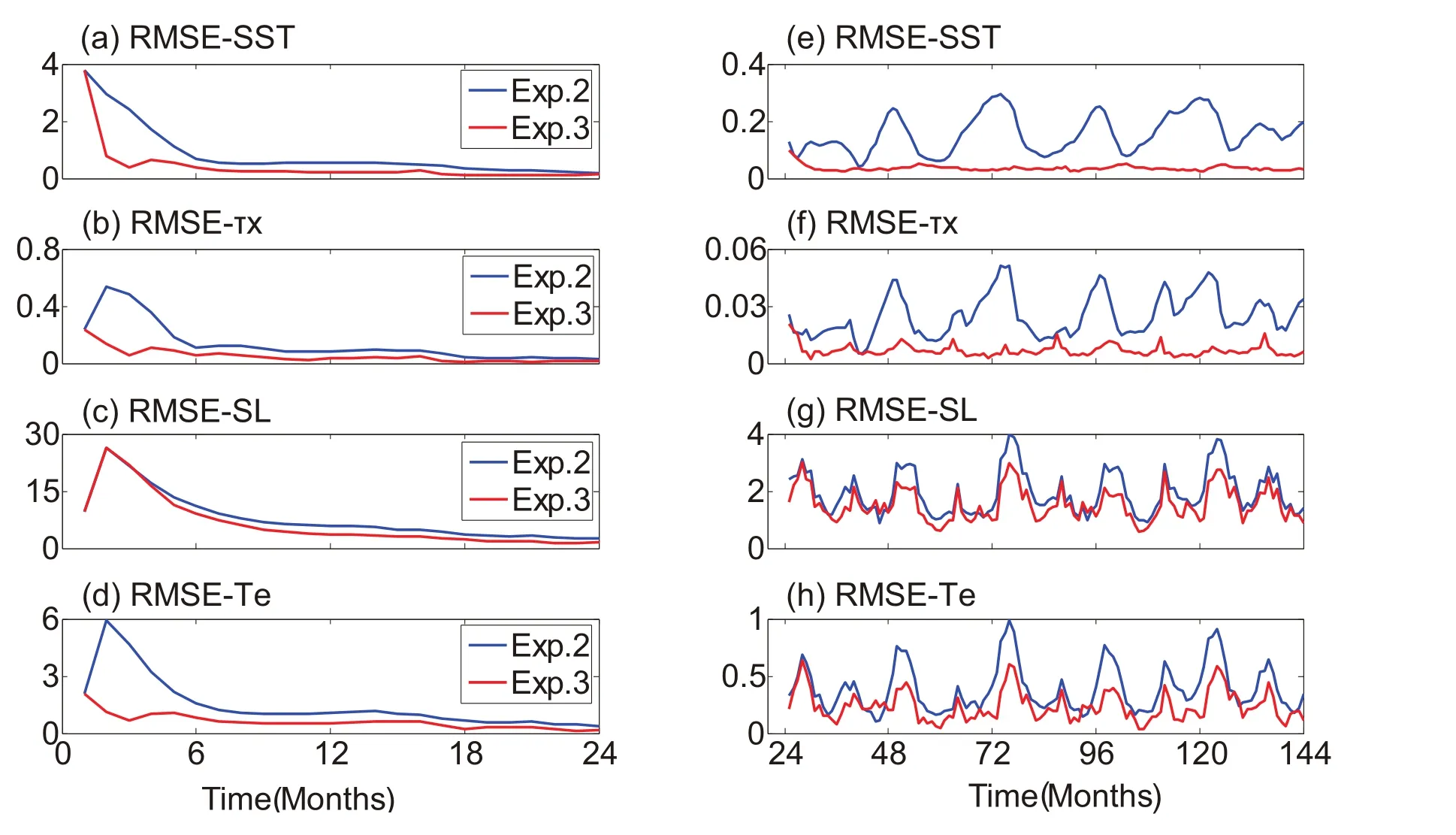
Fig.6.Time series of RMSEs for anomalies of(a,e)SST,(b,f)zonal τ,(c,g)SL and(d,h)Teover the full model domain(30°N–30°S,124°E–78°W).Here,the RMSEs are shown for the first two-year simulations(left-hand panels)and the three-to twelve-year simulations(right-hand panels)from Expt.2(blue)and Expt.3(red),respectively.The RMSEs are calculated on the first day of each month using the corresponding anomalies between Expt.1 and Expt.2 and between Expt.1 and Expt.3,respectively.The units are °C for SST and Te,dyn cm−2for τ,and cm for SL.
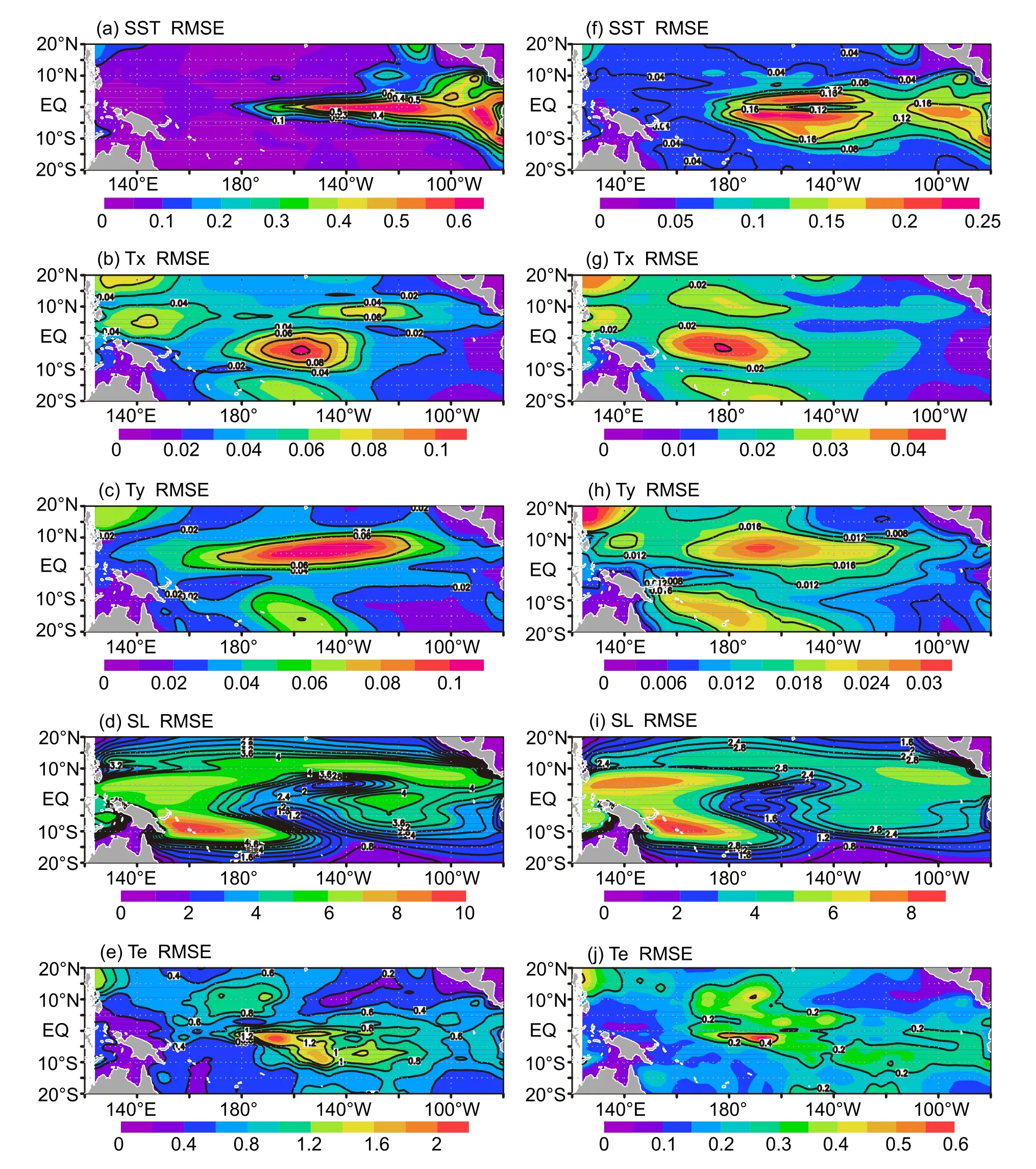
Fig.7.Horizontal distributions of RMSEs for anomalies of(a,f)SST,(b,g)zonal τ,(c,h)meridional τ,(d,i)SL,and(e,j)Te.Here,the RMSEs are calculated from the first 20-year simulations for Expt.2(left-hand panels)and Expt.3(right-hand panels),respectively.The units are °C for SST and Te,dyn cm−2for τ,and cm for SL.
Figure 7 shows the spatial distributions of the RMSEs for the anomalies of SST,zonal wind stress,meridional wind stress,SL and Te.Here,the RMSEs are calculated from Eq.(4)for the first 20-year simulations from Expt.2(left-hand panels)and Expt.3(right-hand panels).The results show that the spatial distributions of the RMSEs for all variables in Expt.3(right-hand panels in Fig.7)are all smaller than those in Expt.2(left-hand panels in Fig.7);whereas,the spatial patterns of the RMSEs are similar to each other in Expt.2 and Expt.3.For the SST field,the regions with maximum RMSE for Expt.2 and Expt.3 are both centered in the central and eastern Pacific;the maximum value is 0.25°C in Expt.3(Fig.7f),which is smaller than that in Expt.2 at 0.66°C(Fig.7a).For the zonal wind stress field,the larger RMSE regions are located in the central equatorial Pacific,with a maximum value of 0.1 dyn cm−2(1 dyn cm−2=0.1 N m−2)for Expt.2(Fig.7b)and0.042dyncm−2Expt.3(Fig.7g).For the meridional wind stress,the RMSEs have the same spatial pattern in Expt.2 and Expt.3,with a maximum value of 0.095 dyn cm−2in Expt.2(Fig.7c)and 0.032 dyn cm−2in Expt.3(Fig.7h).For the SL,the maximum RMSE values are 9 cm and 8 cm,with similar spatial distribution patterns for Expt.2(Fig.7d)and Expt.3(Fig.7i).For the Tefield,the maximum regions are both centered in the central equatorial Pacific,with a maximum value of 2°C in Expt.2(Fig.7e)and 0.55°C in Expt.3(Fig.7j).This represents a reduction in RMSEs by about 71%in Expt.3 compared with Expt.2.
In general,the RMSE differences in the SST,wind stress and Tefields between Expt.2 and Expt.3 are much larger than those in the SL field.This is because,compared with Expt.2,the model parameter αTeis additionally optimized in Expt.3,leading to a Tefield that is effectively recovered.Since the subsurface thermal effect is very important to the evolution of SST anomalies,the improved Tefield in Expt.3 can further affect the simulation of the SST field.So,the biases in SST between the optimizing experiments and the “truth” field decrease faster in Expt.3 than in Expt.2.Thus,the modeled SST field is more likely to recover in Expt.3 compared with Expt.2.Furthermore,the wind stress anomaly field is constructed based on the relationship between the anomalies of SST and wind stress(τ):τ= ατFτ(SST).Therefore,the optimized SST field further improves the simulation of the wind stress anomaly.However,the SL anomaly field needs to be adjusted through dynamic processes when assimilating SST data in the ICM.Consequently,even though the SL field is adjusted to recover to its “truth”field,the biases between the optimizing experiments and the“truth” field are still large compared with other fields.
All in all,additionally optimizing the model parameter αTeusing the 4D-Var assimilation of SST data in the ICM can effectively recover the simulation of major variables,especially for the Te,SST and wind stress fields.Simulation errors induced by biases in the model parameter can be effectively reduced by optimizing the parameter estimation using the 4D-Var method.As such,the optimization procedure can produce an adequate initial condition and model parameter that can be used for ENSO predictions.
4.Effect on ENSO prediction
It is clearly illustrated above that optimizing the model parameter αTethrough the 4D-Var assimilation of SST data can effectively recover the ENSO evolution.It is desirable to check if optimizing model parameters can also benefit ENSO forecasting,in combination with optimizing the initial condition.Here,we perform hindcast experiments using the“biased”model with optimized initial conditions and/or the optimized model parameter,αTe.A series of forecast experiments are conducted using the “biased”model during the period from model time 2062/01/01 to 2079/12/01.Two experiments are performed—one with only the initial condition optimized(Expt.2),and the other with both the model parameter(αTe)and initial condition optimized(Expt.3);the optimized initial condition and model parameter obtained on the first day of each month are used in Expt.2 and Expt.3,respectively.Thus,in these experiments,18×12(=216)hindcasts are obtained in total for analysis in each experiment.
Figure 8 shows the time series of the Niño3.4 indices for the“truth”value(green)and hindcasts made at lead times of three months(Fig.8a),six months(Fig.8b)and nine months(Fig.8c)using the initial conditions and parameter obtained from Expt.2(blue)and Expt.3(red).The hindcast results indicate that the evolution can be predicted very well.As the hindcast time extends,the hindcast errors increase.When optimizing the initial conditions only in Expt.2,the hindcast results exhibit some biases compared with the “truth” field.When optimizing both the initial conditions and the model parameter in Expt.3,it is evident that the Niño3.4 indices produced closely follow the “truth”value.So,additionally optimizing this model parameter can contribute to further improvement in ENSO prediction.Quantitatively,the RMSEs of the Niño3.4 indices predicted in Expt.2 and Expt.3 at the six-month lead time with the “truth”value reduce from 0.47 to 0.06.As the constructed observation error type is simple in this idealized configuration context,the Niño3.4 indices in Expt.3 are almost the same as the“truth”value.
5.Conclusion and discussion
The IOCAS ICM used in this study still suffers from large biases in its real-time ENSO prediction. There are many ways to improve its performance.Previously,we developed a 4DVar data assimilation system for the ICM.As an application,the system was used to optimize the initial conditions for improved ENSO simulation and prediction.Because errors in model parameters are also important sources of model biases,in this paper,the 4D-Var system is used to demonstrate the feasibility of optimizing model parameters for improving ENSO analyses.
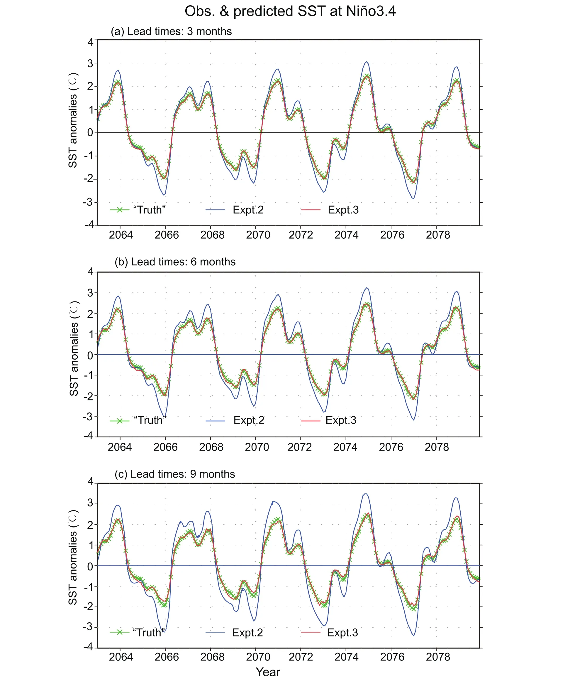
Fig.8.Time series of the Niño3.4 indices for the“truth”model(green)and for hindcasts made using optimized initial conditions in Expt.2(blue)and the additionally optimized model parameter in Expt.3(red)at lead times of(a)three months,(b)six months and(c)nine months.The experiments are performed from model time 2063/01 to 2079/12.
In this ICM,Teis used explicitly to represent the thermocline effect on SST(referred to simply as “the thermocline effect”),and a related parameter(αTe)is introduced to indicate the intensity of the thermocline feedback.In this paper,this model parameter,i.e.αTe,is used as an example to demonstrate the optimization of parameter estimates using the 4D-Var assimilation of SST data in the ICM.To this end,a twin-experiment approach is adopted with an idealized setting.
Results from experiments having only the initial condition optimized and having both the initial condition plus the additional model parameter optimized are compared.As demonstrated before,the simulation and prediction of ENSO can be improved by optimal initialization using the 4D-Var assimilation of SST data in the ICM.Here,it is shown that ENSO evolution can be more effectively recovered by including the additional optimization of this parameter.Through optimizing this parameter,the reduction in RMSEs for anomalies of SST,wind stress,SL and Tetakes place relatively faster compared with that of SL.This is mainly because optimizing the model parameter αTecan effectively improve the simulation of the Tefield.As the subsurface thermal effect is important to SST evolution,the optimized Tefield leads to improved SST depictions.Additionally,the wind stress field is calculated as a response to the SST anomaly using its statistical model;thus,the wind stress anomaly is also improved in the optimized experiment.Since the SL field needs to be adjusted through dynamic processes when SST data are assimilated through the 4D-Var method,this field is less effectively improved.Thus,it is clearly evident that optimizing the model parameter using the 4D-Varbased assimilation of SST data can further improve the simulation and prediction of ENSO.The demonstrated feasibility of optimizing model parameters and initial conditions together through 4D-Var assimilation provides a modeling platform for ENSO studies.
Another application of the 4D-Var data assimilation system implemented in IOCAS ICM to improve its ENSO modeling by optimizing model parameter estimates in the ICM is demonstrated in this paper.The results are obtained in the context of a twin experiment,and these idealized experiments are intended for demonstration purposes.Although only one parameter is considered for the optimized experiments under the idealized setting,it provides a theoretical demonstration and practical assimilation procedure to optimize model parameters.Further applications are underway using the 4DVar data assimilation technique.For example,the ICM’s performance is also sensitive to many other model parameters,including the coupling coefficient between interannual anomalies of SST and wind stress(ατ),the vertical diffusivity coefficient(Kv),the thermal damping coefficient for SST anomalies(λ),and so on.Thus,multi-parameter optimization procedures should be taken into account.Also,some potential problems may exist when applying this technique for fitting a model(which is necessarily biased)to real observed data.In particular,the parameter estimates may not converge as cleanly as shown in Fig.3,and the simultaneous estimation of multiple parameters may be difficult because multiple minima may emerge when estimating the cost function.Also,the spatial structure of the model parameters should be considered.Clearly,more experiments with respect to multi-parameter optimization need to be conducted.Additionally,the subsurface thermal state has considerable influence on the SST in the tropical Pacific.Thus,it is necessary to assimilate subsurface thermal fields into the ICM in addition to the SST data.For example,sea level and horizontal ocean current data need to be considered in the data assimilation procedure.Ultimately,such a combined assimilation of multiple variables and parameters should be considered when using the ICM.
The resultant insight into this predictive understanding and the methodology gained from this work will be transferred to the improvement of real-time ENSO prediction using the IOCAS ICM(Zhang and Gao,2016b).Ultimately,all these efforts are expected to improve ENSO forecasting skill in IOCAS ICM by using the 4D-Var data assimilation system for various data(SST,SL,and others)and various model parameters(αTe,ατ,and others).
Also,other data assimilation methods are currently available,including the EnKF method(Wu et al.,2016).It would be desirable to compare the advantages and disadvantages be-tween these methods in terms of ENSO simulation and prediction.In addition,the adjoint model of the 4D-Var data assimilation equipped with IOCAS ICM provides a way to calculate the gradient of the cost function;the adjoint method with the 4D-Var data assimilation system will be combined with the CNOP(conditional nonlinear optimal perturbation)approach(Mu and Duan,2003)to identify the error structure of initial conditions and model parameters(Tao et al.,2017).More results will be presented in future publications.
Acknowledgements.We would like to thank Drs.Mu MU and Shaoqing ZHANG for their comments.We also wish to thank the anonymous reviewers for their insightful comments and constructive suggestions.This research was supported by the National Natural Science Foundation of China(Grant Nos.41705082,41475101,41690122(41690120)),a Chinese Academy of Sciences Strategic Priority Project—the Western Pacific Ocean System(Grant Nos.XDA11010105 and XDA11020306),the National Programme on Global Change and Air–Sea Interaction(Grant Nos.GASI-IPOVAI-06and GASI-IPOVAI-01-01),the China Postdoctoral Science Foun-dation,and a Qingdao Postdoctoral Application Research Project.
Ballester,J.,D.Petrova,S.Bordoni,B.Cash,M.García-Díez,and X.Rodó,2016:Sensitivity of El Niño intensity and timing to preceding subsurface heat magnitude.Scientific Reports,6,36344,https://doi.org/10.1038/srep36344.
Bjerknes,J.,1966:A possible response of the atmospheric Hadley circulation to equatorial anomalies of ocean temperature.Tellus,18,820–829,https://doi.org/10.1111/j.2153-3490.1966.tb00303.x.
Chen,D.,M.A.Cane,A.Kaplan,S.E.Zebiak,and D.Huang.,2004:Predictability of El Niño over the past 148 years.Nature,428,733–736,https://doi.org/10.1038/nature02439.
Courtier,P.,J.N.Thépaut,and A.Hollings worth,1994:A strategy for operational implementation of4D-Var,using an incremental approach.Quart.J.Roy.Meteor.Soc.,120,1367–1387,https://doi.org/10.1002/qj.49712051912.
Dommenget,D.,and D.Stammer,2004:Assessing ENSO simulations and predictions using adjoint ocean state estimation.J.Climate,17,4301–4315,https://doi.org/10.1175/3211.1.
Gao,C.,and R.-H.Zhang,2017:The roles of atmospheric wind and entrained water temperature(Te)in the second-year cooling of the 2010-12 La Niña event.Climate Dyn.,48,597–617,https://doi.org/10.1007/s00382-016-3097-4.
Gao,C.,X.R.Wu,and R.-H.Zhang,2016:Testing a four-dimensional variational data assimilation method using an im-proved intermediate coupled model for ENSO analysis and prediction.Adv.Atmos.Sci.,33(7),875–888,https://doi.org/10.1007/s00376-016-5249-1.
Huang,R.H.,R.H.Zhang,and B.L.Yan,2001:Dynamical effect of the zonal wind anomalies over the tropical western Pacific on ENSO cycles.Science in China Series D:Earth Sciences,44,1089–1098,https://doi.org/10.1007/BF02906865.
Kalnay,E.,2003:Atmospheric Modeling,Data Assimilation and Predictability.Cambridge University Press,342 pp.
Liu,D.C.,and J.Nocedal,1989:On the limited memory BFGS method for large scale optimization.Mathematical Programming,45,503–528,https://doi.org/10.1007/BF01589116.
Liu,Y.,andH.-L.Ren,2017: ImprovingENSO prediction in CFSv2 with an analogue-based correction method.International Journal of Climatology,37(15),https://doi.org/10.1002/joc.5142.
Liu,Y.,Z.Liu,S.Zhang,R.Jacob,F.Lu,X.Rong,and S.Wu.,2014:Ensemble-based parameter estimation in a coupled general circulation model.J.Climate,27,7151–7162,https://doi.org/10.1175/JCLI-D-13-00406.1.
Lu,J.X.,and W.W.Hsieh,1998:On determining initial conditions and parameters in a simple coupled atmosphere–ocean model by adjoint data assimilation.Tellus A,50,534–544,https://doi.org/10.3402/tellusa.v50i4.14531.
Mu,M.,and W.S.Duan,2003:A new approach to studying ENSO predictability:Conditional nonlinear optimal perturbation.Chinese Science Bulletin,48,1045–1047,https://doi.org/10.1007/BF03184224.
Mu,M.,W.S.Duan,and C.J.Wang,2002:The predictability problems in numerical weather and climate prediction.Adv.Atmos.Sci.,19,191–204,https://doi.org/10.1007/s00376-002-0016-x.
Mu,M.,W.Duan,Q.Wang,and R.Zhang,2010:An extension of conditional nonlinear optimal perturbation approach and its applications.Nonlinear Processes in Geophysics,17,211–220,https://doi.org/10.5194/npg-17-211-2010.
Peng,S.-Q.,and L.Xie,2006:Effect of determining initial conditions by four-dimensional variational data assimilation on storm surge forecasting.Ocean Modelling,14,1–18,https://doi.org/10.1016/j.ocemod.2006.03.005.
Peng,S.Q.,Y.N.Li,and L.Xie,2013:Adjusting the wind stress drag coefficient in storm surge forecasting using an adjoint technique.J.Atmos.Oceanic Technol.,30,590–608,https://doi.org/10.1175/JTECH-D-12-00034.1.
Ren,H.-L.,Y.Liu,F.-F.Jin,Y.P.Yan,and X.W.Liu,2014:Application of the analogue-based correction of errors method in ENSO prediction.Atmospheric and Oceanic Science Letters,7,157–161,https://doi.org/10.3878/j.issn.1674-2834.13.0080.
Tao,L.-J.,R.-H.Zhang,and C.Gao,2017:Initial error-induced optimal perturbations in ENSO predictions,as derived from an intermediate coupled model.Adv.Atmos.Sci.,34,791–803,https://doi.org/10.1007/s00376-017-6266-4.
Wang,B.,X.L.Zou,and J.Zhu,2000:Data assimilation and its applications.Proceedings of the National Academy of Sciences of the United States of America,97(21),11 143–11 144,https://doi.org/10.1073/pnas.97.21.11143.
Wu,X.R.,S.Q.Zhang,Z.Y.Liu,A.Rosati,T.L.Delworth,and Y.Liu,2012:Impact of geographic-dependent parameter optimization on climate estimation and prediction:Simulation with an intermediate coupled model.Mon.Wea.Rev.,140,3956–3971,https://doi.org/10.1175/MWR-D-11-00298.1.
Wu,X.R.,G.J,Han,S.Q.Zhang,and Z.Y.Liu,2016:A study of the impact of parameter optimization on ENSO predictability with an intermediate coupled model.Climate Dyn.,46,711–727,https://doi.org/10.1007/s00382-015-2608-z.
Xie,S.-P.,C.Deser,G.A.Vecchi,J.Ma,H.Y.Teng,and A.T.Wittenberg,2010:Global warming pattern formation:Sea surface temperature and rainfall.J.Climate,23,966–986,https://doi.org/10.1175/2009JCLI3329.1.
Zebiak,S.E.,and M.A.Cane,1987:A model El Niño-southern oscillation.Mon.Wea.Rev.,115,2262–2278,https://doi.org/10.1175/1520-0493(1987)115<2262:AMENO>2.0.CO;2.
Zhang,R.-H.,and C.Gao,2016a:Role of subsurface entrainment temperature(Te)in the onset of El Niñoevents,as represented in an intermediate coupled model.Climate Dyn.,46,1417–1435,https://doi.org/10.1007/s00382-015-2655-5.
Zhang,R.-H.,and C.Gao,2016b:The IOCAS intermediate coupled model(IOCAS ICM)and its real-time predictions of the 2015-2016 El Niño event.Science Bulletin,61,1061–1070,https://doi.org/10.1007/s11434-016-1064-4.
Zhang,R.-H.,S.E.Zebiak,R.Kleeman,and N.Keenlyside,2003:A new intermediate coupled model for El Niño simulation and prediction.Geophys.Res.Lett.,30,2012,https://doi.org/10.1029/2003GL018010.
Zhang,R.-H.,R.Kleeman,S.E.Zebiak,N.Keenlyside,and S.Raynaud,2005a:An empirical parameterization of subsurface entrainment temperature for improved SST anomaly simulations in an intermediate ocean model.J.Climate,18,350–371,https://doi.org/10.1175/JCLI-3271.1.
Zhang,R.-H.,F.Zheng,J.Zhu,and Z.G.Wang,2013:A successful real-time forecast of the 2010-11 La Niña event.Scientific Reports,3,1108,https://doi.org/10.1038/srep01108.
Zhang,S.,M.J.Harrison,A.T.Wittenberg,A.Rosati,J.L.Anderson,and V.Balaji,2005b:Initialization of an ENSO forecast system using a parallelized ensemble filter.Mon.Wea.Rev.,133,3176–3201,https://doi.org/10.1175/MWR3024.1.
Zhang,X.F.,S.Q.Zhang,Z.Y.Liu,X.R.Wu,and G.J.Han,2015:Parameter optimization in an intermediate coupled climate model with biased physics.J.Climate,28,1227–1247,https://doi.org/10.1175/JCLI-D-14-00348.1.
Zheng,F.,J.Zhu,R.-H.Zhang,and G.Q.Zhou,2006:Ensemble hindcasts of SST anomalies in the tropical Pacific using an intermediate coupled model.Geophys.Res.Lett.,33,L19604,https://doi.org/10.1029/2006GL026994.
Zheng,F.,J.Zhu,H.Wang,and R.-H.Zhang,2009:Ensemble hindcasts of ENSO events over the past 120 years using a large number of ensembles.Adv.Atmos.Sci.,26,359–372,https://doi.org/10.1007/s00376-009-0359-7.
猜你喜欢
杂志排行
Advances in Atmospheric Sciences的其它文章
- Validation and Spatiotemporal Distribution of GEOS-5–Based Planetary Boundary Layer Height and Relative Humidity in China
- Effects of Sea-Surface Waves and Ocean Spray on Air–Sea Momentum Fluxes
- Evaluation of TIGGE Ensemble Forecasts of Precipitation in Distinct Climate Regions in Iran
- Evaluating the Capabilities of Soil Enthalpy,Soil Moisture and Soil Temperature in Predicting Seasonal Precipitation
- Large-scale Circulation Control of the Occurrence of Low-level Turbulence at Hong Kong International Airport
- Variations in High-frequency Oscillations of Tropical Cyclones over the Western North Pacific
