Effects of Interfaces on Dynamics in Micro-Fluidic Devices:Slip-Boundaries’Impact on Rotation Characteristics of Polar Liquid Film Motors∗

Su-Rong Jiang(姜素蓉),Zhong-Qiang Liu(刘中强),,† Tamar Amos Yinnon(他玛·阿摩司·依侬), and Xiang-Mu Kong(孔祥木)Department of Physics,Qufu Normal University,Qufu 7365,China

2Kibbutz Kalia,Doar Na Kikar,Jordan 90666,Israel

1 Introduction

Interfacial liquid zones(ILZ)adjacent to membranes,metals or biological tissues,though researched for many years,[1]their study continues to have significant scienti fic and technological consequences.[2−3]For example,the∼ 10−4m wide ILZ(denoted exclusion zone–EZ)in water or other polar liquids adjacent to hydrophilic membranes or reactive metals was recently discovered.[2]

Identifying ILZ’s physical properties often is hindered by diffculties separating the zone’s contribution to observed quantities from those of its adjacent bulk liquid,e.g.,while EZ’s viscosity and density(which are much higher than those of the adjacent bulk liquid)are determinable,their molecular orderings underlying its photonic crystalline properties are not yet known.[2,4]In our search for ways around this hindrance,we recently showed “imprinting” EZ water in bulk water provides insight into the phase transitions leading to its formation.[4]In this paper,we offer an alternative complementary route for studying ILZs,i.e.,examining their impact on the electro-hydro-dynamical(EHD)motions of the recently invented suspended polar liquid film motor(PLFM).[5−6]PLFMs provide good platforms for studying micro-structures of different polar liquid films(including liquid crystal films).[5−8]The PLFM consists of a quasitwo-dimensional electrolysis cell in an external in-plane electric field(see Fig.1).[5−9]Recently,the polar liquid film electric generator,an inverse device of the PLFM,has been created.[10]

In previous studies,we developed models for the PLFMs which enabled quantitative and qualitative explanations for numerous experimental results,[11−12]e.g.,its rotation direction,threshold fields for onset of its EHD motions and the distribution of its angular velocity.The models also enabled a series of predictions–recent experiments verified those pertaining to the EHD rotations and the plastic vibrations of the ACM.[8]

The impact of the PLFM’s film boundaries on its EHD motions hitherto has not been addressed,i.e.,all previous models assumed no-slip hydrodynamic boundary conditions at film borders.[8,11−16]However,experiments show EHD motions in PLFMs,near their films’borders,depend on polar liquid type.For example:a macroscopic observable almost static region exists near the boundary of the rotating N-(4-methoxybenzylidene)-4-butylaniline liquid crystal film;[7]for the rotating 2,5-Hexadione film,the rotation’s linear velocity decreases slowly to zero in the radial direction on approaching the border;a largelinear velocity appears at the border of the rotating Benzonitrile film.[6]Moreover,recent experiments and simulations show:negative slippage exists in hydrophilic microchannels[17]and on interfaces with a strong solid- fluid attraction;[18]numerous no-slip and partial-slip phenomena of polar liquids(e.g.,water)on various solid interfaces were reported;[19]large slip effects(slip length varying from several micrometers(µm)to several hundredsµm)were observed on nanostructured superhydrophobic surfaces.[20−24]

The goal of our study is to investigate effects of interfaces on PLFMs’rotational EHD motions under slip boundary conditions.To the best of our knowledge,our study is the first to theoretically derive slip boundary effects on PLFM’s dynamics.As to its theoretical,experimental and technological significance:Firstly,modeling the EZ’s effects on liquid films has not yet been undertaken. Examining such effects promise elucidating its structure.[2,25]Secondly,EHD motions of liquid crystal films currently are studied intensively and their unique properties are applied widely in industry.[26−29]Thirdly,exploring the impact of interactions between liquids and solids on EHD motions will advance our understanding of lf uid mechanics.Fourthly,slippage on liquid-solid interfaces affects fluid transportation in micro-and nano- fluidic systems:[30]large boundary slip can reduce hydrodynamic drag in micro-and nano-channels,[30−31]improving the detection effciency of the micro- fluidic chips,i.e.,the study of related mechanisms and laws is helpful to accelerate developments of lab-on-a-chip technology.Fifthly,we expect investigations on boundary slippage to elucidate several experimental boundary phenomena in general and of various PLFMs types in particular.Such elucidations are important for delineating optimizing methods for realizing PLFM’s applications in the lab-on-a-chip.

The outline of this paper is as follows:In Sec.2,we present a model for PLFMs with slip boundary conditions,and derive their general solutions describing their EHD motions.In Sec.3,we derive a series of specific characteristics of the DC and the AC PLFMs,and compare these with experimental ones.Our conclusions we present in Sec.4.For convenience,the DC motor(DCM)and the AC motor(ACM)denotations are used to represent the DC and the AC PLFMs,respectively.We stress that in this paper we only theoretically derive characteristics of the DCM and the ACM under slip boundary conditions.We do not report any new experimental data.All the experimental results cited in our paper were obtained by different research groups and reported in the literature.

2 Model of PLFMs with Slip Boundary Conditions and Its Solutions

Our no-slip models of the DCM and the ACM are based on the assumption that a polar liquid film in an external electric field can be depicted as a Bingham plastic fluid with an effective electric dipole moment.[11−12]Quantum electro-dynamic aspects of polar liquids,[32−37]together with experimental results,e.g.,of EZs[2,4]and the floating water bridge,[38−39]underlie this assumption–see Sec.2 in Refs.[11]and[12].Encouraged by our models’previous successes,[11−12]we expand these to slip boundary models.The dynamical equation of the PLFM reads[11−12]

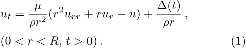
Hereuαanduαα(α=r,t)respectively denote the firstand the second-order partial derivatives of the linear velocityu(r,t)with respect toα.µ,ρ,andR,respectively,are the plastic viscosity,the density and the radius of the liquid film.

whereε0,εr,andτ0,respectively,are the dielectric constant of the vacuum,the relative dielectric constant and the yield stress of the liquid film;Eext(t)andEel(t)are,respectively,the magnitudes of the external electric field Eextand of the electrolysis electric field Eelat timet;As shown in Fig.1,θEJis the angle between Eextand Eel.Generally,θEJ=π/2.µ,ρ,εrandτ0of an ILZ and of its adjacent liquid may significantly differ,with the differences impinging on boundary slip.

For slip-boundary models,besides the initial conditionu(r,t)|t=0=0 and a natural boundary conditionu(r,t)|r=0=0,Eq.(1)should also satisfy a slip-boundary condition

Hereusis a nonzero slip velocity.lssymbolizes the slip length resulting from the interface’s impact onµ,ρ,εrandτ0.(Navier was the first to define slip lengths;[40]nowadays it customarily is used to characterize the type of slip flows in channels,[41−43]e.g.,in micro-or nano-channels in lab-on-a-chip devices.)For a transverse cross section of an in finite long cylindrical channel,lsis the extrapolated distance relative to its wall where the tangential velocity component vanishes(see Fig.2(c)).[40−41]Negativeslip,no-slip,partial-slip and perfect-slip conditions are described with differentlsvalues(see Fig.2):if−Rc＜ls＜0,withRcdenoting the radius of the cylinder,the flow is negative slip flow(i.e.,locking boundary),[43−44]see Fig.2(a);ifls=0,the flow is stick flow(i.e.,no slip boundary),see Fig.2(b);ifls=∞,the flow is plug flow(i.e.,perfect slip boundary),see Fig.2(d);intermediate values oflsrepresent partial slip flow,see Fig.2(c).We stress that the boundary zone with the negative linear velocity in Fig.2(a)does not represent the existence of a reverse flow;it may be considered as an approximately static liquid zone.[43]With the PLFM’s suspended film corresponding toa∼102nm thick slice of a cylindrical channel,in our model we adopt the aforementioned definitions ofls.The film’s schematic profiles with abovedefined boundary conditions are plotted in Fig.3.Its denotations are the same as those used in Fig.2.

Fig.1 (Color online)Schematic picture of the PLFM operated with DC fields.The device consists of a two dimensional frame with two graphite(or copper)electrodes(gray strips)on the sides for electrolysis of the liquid film(blue-green zone).The radius and diameter of the film are denoted,respectively,as R and D.The frame is made of an ordinary blank printed circuit board with a circular(or square)hole at the center.The diameter of the hole may vary from several centimeters to less than a millimeter.Suspended liquid films as thin as hundreds of nanometers or less may be created by brushing the liquid on the frame.The electric current Jel(induced by electrolysis field Eel)and an external electric field Eext are produced by two circuits with voltage Ueland Uext,respectively.Eext,induced by two plates(striate strips)of a large capacitor,is perpendicular to Jel.When the magnitudes of Eeland Eextare above threshold values,the film rotates,i.e.,constitutes a motor.The rotation direction obeys a right-hand rule,i.e.,Eext×Jel.If the DC electric sources(bold vertical lines in circuits)are replace by AC ones,PLFM can also rotate in AC fields with the same frequencies.

To explicate the physical quantities affecting EHD motions,we transform to dimensionless variables.ChoosingR,µ,andρas basic parameters,letting

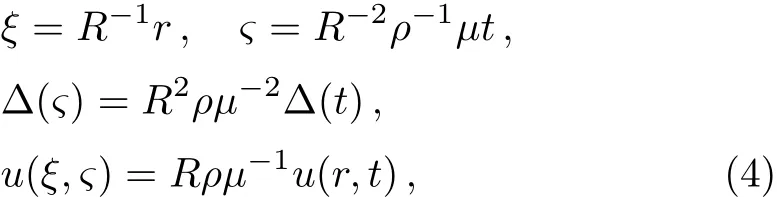
withRandtc=R2ρµ−1the characteristic length and characteristic time,respectively.Letk=ls/R,Eq.(1),its initial and boundary conditions transform into dimensionless equations,i.e.,

The general solutions of Eq.(5)can be obtained by the method of eigenfunctions.[45]Assumingu(ξ,ς)=Rf(ξ)T(ς),inserting it into the homogeneous equation of Eqs.(5a)and(5b),respectively,we obtain the eigenvalues problem

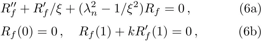
where separation of variables method[45]was used to introduce eigenvaluesλn.The eigenfunctions of Eq.(6),depicting the spatial modes in the general solutions of Eq.(5a),are a series of the ordinary Bessel functions of order one:J1(λnξ),ξ⊆ [0,1],n=1,2,...Obviously,J1(λnξ)satisfy the first boundary condition in Eq.(6b)and the corresponding eigenvaluesλnare determined by

which is a natural result whenJ1(λnξ)satisfy the second boundary condition in Eq.(6b).For a givenk,λncan be obtained numerically from Eq.(7).With the values ofλngoverning the behaviors ofJ1(λnξ),which reflect the spatial modes of the rotating liquid film,Eqs.(6b)and(7)display that the rotation properties of PLFMs with the slip boundary conditions depend onk,i.e.,on the ratio oflsandRbut not on their independent values.

From Eqs.(6)and(7),it may be proved thatJ1(λnξ)should obey the following orthogonality relations(see Appendix A)

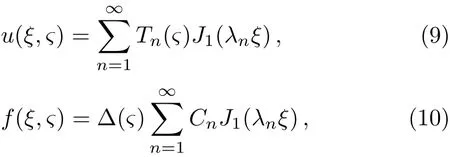
whereδmn=1 whenm=n,δmn=0 whenm/=n.Since the above Bessel function series is a complete orthogonal system,the general solution to Eq.(5a)and the last termf(ξ,ς)= Δ(ς)/ξin Eq.(5a)may be expanded by them in generalized Fourier series,i.e.,

with

Fig.2 Schematic transverse cross-sections of an in finite long cylindrical channel filled with liquid,with slip boundary conditions described by different slip lengths ls.Rcdenotes the channel’s radius.(a)For −Rc ＜ ls ＜ 0,the liquid’s linear velocity in the channel,i.e.,uc(r,t)(represented with orange arrows)as a function of r quickly diminishes to zero in the liquid near the boundary if there is negative slip at the liquid-solid interface.Pink dotted arrows denote an imaginary reverse flow.(b)For ls=0,uc(r,t)gradually diminishes to zero near the boundary if there is no slip at the solid-liquid interface,i.e.,us=0.(c)For 0＜ls＜∞,when boundary slip occurs at the solid-liquid interface,there is relative velocity between fluid flow and the cylinder boundary,i.e.,us＞0.(d)For ls=∞,the solid-liquid interface does not exert any resistance on the fluid,i.e.,uc(r,t)is independent of r and us=uc(r,t).The horizontal dash-dot lines and the horizontal dotted lines represent the central line of channels and the no-slip surfaces,respectively.

Inserting Eq.(9)into Eq.(5b),one finds that the first boundary condition of Eq.(5a)is satis fied automatically and the second one yields Eq.(7).Inserting Eqs.(9)and(10)into Eqs.(5a)and(5c),respectively,we have

andTn(0)=0.The general solution to Eq.(12)is

where the constantQnis determined byTn(0)=0.

Equations(9)and(13)present our model’s general dimensionless solutions for PLFMs under slip boundary conditions.The linear velocity distribution of rotating PLFMs is given by Eq.(9),in which the spatial modes and the time factors are respectively depicted byJ1(λnξ)satisfying Eqs.(7),(8)and Eq.(13).The corresponding dimensionless angular velocity is given byω(ξ,ς)=u(ξ,ς)/ξ.From Eq.(4),one can obtain the linear velocityu(r,t),and the corresponding angular velocity

3 Results and Discussion

PLFMs can work perfectly with many different crossing electric fields, e.g., DC,[5−6,11]AC[5,12]squarewave,[13]and other type.[14]In this study,we present the boundary slip effects on the rotation properties of DCM and ACM,and compare these with experimental results.

3.1 DCM with Slip Boundary Conditions

According to Eq.(2),for DCM Δ(t)is a constant,i.e.,

From Eqs.(4),(13),and(15),we obtain the time factors describing the rotation evolution of the DCM:

where Δdc(ς)=R2µ−2ρΔdc.Combining Eqs.(9),(11),and(16),we obtain the dimensionless linear velocity of the DCM

where

Equation(17)indicates:

(i)The rotation speed is proportional to Δdc.

(ii)ς=t/tcandtc=R2ρ/µshow that for largeR,highρand lowµ,it takes a long time for the DCM reaching the steady rotation state.The physical reason is that largeRresults in momentum exchange within a large liquid region,highρreflects the film’s large inertia and lowµslows down the momentum exchange in the liquid film.

(iii)The spatial modes of the film’s rotation depend onλn.

(iv)kaffects the rotations,reflecting the interface’s impact on the film’s EHD motions.

To illuminate dynamical characteristics for differentkvalues,we adopt the experimental parameters of the exemplary extensively measured and theoretically investigated DCM,[5−6,11−12]i.e.:ε0=8.85 × 10−12F·m−1,εr= 80,EextUelsinθEJ= 7.2 × 106V2·m−1,R=1.55 × 10−2m,ρ=103kg·m−3,µ=10−3Pa·s and its derivedτ0=6.77 × 10−5Pa.With these parameters,characteristics of the angular and linear velocities dependencies onkwere investigated.It is found that by settingk= −0.1,10−3,1 or 103,the DCM rotates under,respectively,negative-slip,approximately-no-slip,partialslip and approximately-perfect-slip boundary conditions,as discernible from Fig.4:This figure depicts the profiles of our computed angular and linear velocities at different times–by drawing the intersection points of the tangent lines to the curves witht=1000 s at the pointR(i.e.,ξ=1)and the horizontal axis in the insets of Fig.4,it is noticeable that Figs.4(a)–4(d)are consistent with the four slip boundary cases presented by Figs.3(a)–3(d),respectively.To illustrate this more clearly,we plot the profiles and maxima of the steady rotation linear velocities in Fig.5.The main features observable from Figs.4 and 5,are:

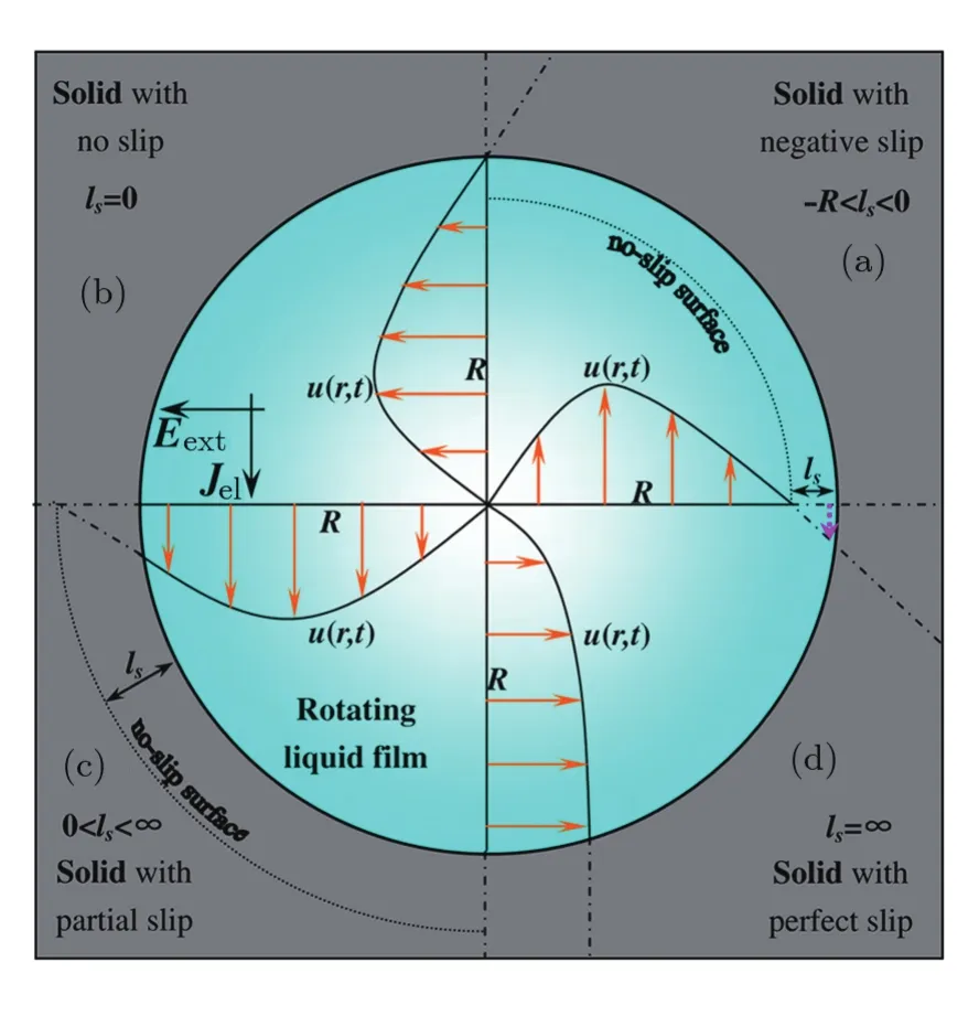
Fig.3 Schematic linear velocity’s profiles of the slip boundary conditions,with different slip lengths lsin a rotating liquid film. (a)−R ＜ ls＜ 0,negative-slip boundary;(b)ls=0,no-slip boundary;(c)0＜ls＜∞,partial-slip boundary;(d)ls=∞,perfect-slip boundary.

(i)For anyk,the points near the center of the film start to rotate earlier than those farther away from it,and the angular velocities decrease with increasingr(orξ) –see Fig.4.These results are in full agreement with the experimental ones.[5−7]

(ii)Askincreases,the angular velocity of the steady rotation grows gradually and its decay rate withrdeceases slowly.Experiments capable of verifying this prediction have not yet been reported and are called for.

(iii)The linear velocity’s spatial distribution depends onk.

(a)For−1/2＜k＜0,the DCM rotates under a negative slip boundary condition,[46]i.e.,locking boundary–see Fig.4(a),which shows that asrincreases from zero the rotation’s linear velocity increases quickly from zero to a maximum and then decreases slowly to zero,even to a negative value asrincreases further.

As mentioned in Sec.2,the zone around a border with negative linear velocity(see pink dashed arrows in Figs.2(a)and 3(a))may be considered as a zone with static liquid. Simulation with the lattice Boltzmann method show that a strong solid- fluid attraction may result in a small negative slip length.[18]Molecular dynamics simulations show that the no-slip or locking boundary conditions correspond to ordered liquid structures close to the solid walls leading to zero and negative slip lengths,respectively.[47]Strong solid- fluid attractions and ordered liquid structures close to solid walls have been observed in numerous recent experiments,such as the millions molecules wide EZ with its long-range molecular orderings,high-viscosity and liquid-crystal-phase properties discernible in polar liquids adjacent to objects like biological tissues,optical fibers,gels with charged or uncharged surfaces,reactive metal sheets and hydrophilic membranes(e.g.,Na fion).[2]

Combining the experimental and simulations’results cited in the last paragraph with our theoretical ones,we predict that the DCM may exhibit a physics picture given by Fig.4(a)when motor’s frames are made of hydrophilic,biological or reactive metals materials.This conjecture is partly supported by the experimental results of rotating liquid crystal films driven by crossing DC electric fields:Figure 4(a)in this paper is qualitatively consistent with Figs.2(d)and 5 in Ref.[7].Since water and liquid crystals have different micro-structures and properties,further experiments are called for to verify the above prediction and more detailed theoretical investigations are needed.

(b)Forka small positive number,e.g.0＜k≤ 10−2,the DCM rotates under an approximately-no-slip condition – Fig.4(b)and the curve withk=10−2in Fig.5 show that the rotation properties of the DCM are almost the same as those obtained on assuming no slip boundary condition,see Figs.7 and 8 of Ref.[11].The linear velocity has its maximum atR/e,witherepresenting the Euler number,and the angular velocity is a decreasing function of the radiusr.This result shows that the slip boundary effect may be ignored when the slip lengthlsis much less than the size of the liquid film.It is consistent with the characteristics of the rotating 2,5-Hexadione film.[6]It also indirectly proves that our model is reasonable.

(c)For 10−2＜k＜∼10,the DCM rotates under partial slip condition.Askincreases above 10−2,the maximum value of the linear velocity of the steady rotating liquid film increases and its location moves fromR/etoR,as shown in Fig.5.

It is noteworthy that fork=1 andt=1000 s,the maximum value of the linear velocity locates around 2R/e,the angular velocity decays slowly with increasingrand it has a large value at the boundary(see Fig.4(c)).These properties are qualitatively consistent with the experimental ones exhibited by the rotating Benzonitrile film(see Fig.3(c)in Ref.[6]).Hence investigating the slip boundary effects facilitates understanding some experimental results unexplainable with our previous no-slip model.[11]

(d) For suffcient largek,e.g.,k≥ 10(see the inset in Fig.5(a)),the DCM rotates under approximatelyperfect-slip boundary conditions.The angular velocity is a decreasing function of the radiusr(see Fig.4(d)),but the linear velocity of steady rotation is an increasing function of the radiusr(see the inset in Fig.4(d)).To the best of our knowledge,hitherto,there are no corresponding experimental results for verifying these theoretical ones.

Fig.4 The profiles of the angular velocity of the DCM with four different boundary conditions represented by different values of k at different times:(a)k= −0.1;(b)k=10−3;(c)k=1;(d)k=103.The insets show the profiles of the corresponding linear velocity of each figure.

3.2 ACM with Slip Boundary Conditions

Experimental[5,8]and our previously published theoretical results[12]show:when the crossing AC fields have the same frequencies,the ACM exhibits rotation characteristics similar to those of the DCM;AC fields with different frequencies can merely induce vibrations not rotation.Our detailed previously published predictions on ACM’s rotation and vibration characteristics[12]are now fully con firmed by experiments,[8]with the exception of some details of the elastic vibration–a model based on our previous published one,with the improvement of assuming the film to be an elastic Bingham fluid,explains these details.[8]In the model presented in this paper,we did not include the aforementioned improvement,i.e.,we do not expect it to describe all vibration properties of ACMs.Still,based on its previous success in correctly describing ACMs’rotation properties,we conjecture our model can elucidate the effect of slip boundaries on the ACM rotations.

For the analysis we define the alternating external electric field and electrolysis voltage,respectively,as

HereE0andU0,respectively,denote the amplitudes of the electric field and the voltage,ωac=2πfrepresents their angular frequencies,φis the initial phase of the electrolysis voltage and it also represents the phase difference between the AC fields.From Eq.(2),the source driving the rotation of the ACM is(as explicitly shown in Ref.[12]–Subsec.3.2)

where

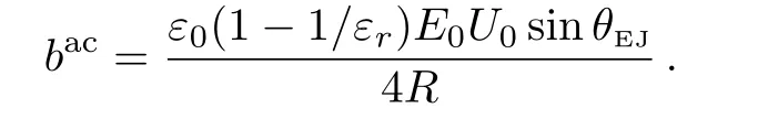
Equation(18)is suitable for studying the rotation of the ACM only ifBc＞0,which means that the active torque can continuously destroy the plastic structure of the liquid film to induce rotation.Combining Eqs.(4),(9),(13)with Eq.(18),one may derive the dimensionless linear velocity of the ACM,i.e.,

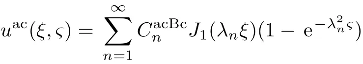
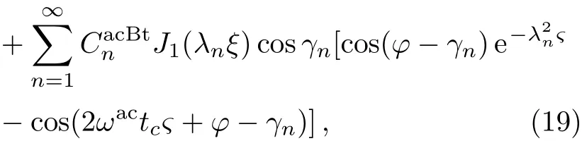
where

And then the corresponding angular velocity is given by Eq.(19)andω(ξ,ς)=u(ξ,ς)/ξ.

Fig.5 The profiles of the angular velocity of the steady rotating DCM and ACM with different k values.k varies from −0.1 to 103.(a)DCM;(b)ACM with f=50 Hz and φ =0;(c)ACM with f=0.5 Hz and φ =0;(d)ACM with f=0.5 Hz and φ =5π/12.The insets show the profiles of the corresponding linear velocity of each figure.Obviously,the rotation properties of the DCM depend on k,while those of the ACM are associated with k as well as these depend on the frequencies and on the phase difference of the AC fields.

Equation(19)indicates that for the ACM,rotation of the film comprises both the rotational modes and the plastic-vibration modes.Our calculations,reported in the following paragraphs,show the contributions of these two different types of modes vary with the magnitudes,the frequencies and the phase difference of the AC fields.Thus,the dynamical characteristics of the ACM with slip boundary conditions depend onkas well as on the aforementioned variables.

To illuminate in detail the dynamical characteristics of the ACM for differentk,f(f=ωac/2π)andφvalues,we adopt in the expression forbac(employed in Eq.(18))E0U0sinθEJ=7.2×106V2·m−1;for the other parameters we adopt the values of the DCM of Subsec.3.1.Employing Eqs.(4),(14),and(19),we computed numerous profiles of the angular velocity of the steady rotating ACM for differentk,fandφvalues and in depth analyzed these.Exemplary cases,which depict the main trends,were plotted in Figs.6,7,and 8.From those we learn:

(i)The boundary dynamical behaviors of the ACM,just as those of the DCM studied earlier in Subsec.3.1,are determined byk.On comparing Fig.6 with Fig.3,it is discernible that askincreases ACM subsequently exhibits“negative”-, “no”-, “partial”-,and “perfect”-slip behaviors.Moreover,the maximum of rotation linear velocity increases and its location approaches the film’s border askincreases,see Fig.7.To the best of our knowledge,neither experimental nor computational data have been reported that can verify Figs.6 and 7’s predictions.

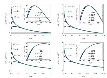
Fig.6 The profiles of the angular velocity of the steady rotating ACM with different values of f for φ =0 at time t=1000 s.f varies from 0.05 Hz to 500 Hz.(a)k= −0.1;(b)k=10−3;(c)k=1;(d)k=103.The insets show the profiles of the corresponding linear velocity of each figure.Obviously,the rotation properties around the film’s center depend on f,while those near the film’s boundary are associated with k.As f decreases,the angular velocities vary from a monotonically decreasing function to a first increasing then decreasing function.As k increases,the ACM subsequently exhibits negative-slip,no-slip,partial-slip,perfect-slip behaviors.

(ii)For given AC fields’magnitudes,the contributions of rotation modes and plastic vibration modes depends onfandφ:

(a)For highfand smallφ,e.g.,f≥ 50 Hz andφ=0,the ACM exhibits characteristics similar to those of the DCM:All the angular velocities are almost monotonically decreasing functions ofrand all the linear velocities increase with increasingk–compare Fig.6 with Fig.4.These theoretical results agree well with the experimental ones.[5]

(b)fmainly affects the rotational properties around the film’s center– see Fig.6.Asfdecreases,the ACM and the DCM exhibit different properties.The angular velocities of the ACM do not monotonically decrease withr,as do those of the DCM–this can be seen by comparing Fig.4 with Fig.6.The ACM’s angular velocities increase first and then decrease asrenhances.Moreover,the location of the maximum of the angular velocity moves away from the center of the liquid film asfdecreases.The underlying physical reason for this dependency of the ACM’s angular velocities onris that the contributions of the plastic vibration modes to the linear velocity increase as AC fields’frequencies decrease.When the frequencies are higher,the minor and faster plastic vibrations,arising from the second term of Eq.(18),can not induce a macroscopic flow in the liquid film in each half period ofT1=1/(2f).Asfdecreases,the plastic vibration modes’ability to produce a macroscopic reverse flow in the liquid film strengthens and leads to the velocities presented in Fig.6.These theoretical results agree well with the numerical ones given in Fig.6 of Ref.[8],which show that as frequencies increase,the plastic vibration gets weaker.

Fig.7 The profiles of the angular velocity of the rotating ACM with different k values for various values of φ(φ =0,π/6,π/4,π/3,5π/12)at time t=1000 s:(a)k= −0.1;(b)k=10−3;(c)k=1;(d)k=103.The frequencies of the AC fields are 50 Hz.The insets show the profiles of the corresponding linear velocity of each figure.Obviously,the angular velocities are decreasing functions of the radius.On comparing curves in this figure with those with t=1000 s in Fig.4,for the corresponding k values,one finds that the ACM and the DCM exhibit similar characteristics when AC fields’frequencies are large(e.g.,f=50 Hz).As φ increases,the rotation speed decreases gradually.

(c)As to effects ofφon the rotation characteristics of the ACM,its rotation speed decreases asφincreases–see Fig.7.The underlying reason is that asφincreases,Bc=(baccosφ−2τ0)in Eq.(18)decreases.This leads to a diminishment of the rotation modes’contributions to the EHD motions in the ACM,while those of vibration modes become more distinct.Moreover,whenfis high enough,the positional deviation of the maximum of the angular velocity from the center of the film is negligible with increasingφ.However,whenfis small,e.g.,f=0.5 Hz,this deviation becomes significant asφincreases:Whenφis large enough,the region near the center of the film and that near the border may rotate in opposite directions(see Fig.8).The aforementioned theoretical results agree with the experimental and calculated ones:Experimental results show that average tangential velocities of an ACM,with a phase difference ofφ=5π/12,frequency of 41 Hz andEext0Eel0=2.2×108V2·m−2,may be positive or negative–see Fig.3 in Ref.[18];Calculated results of shear rates show that the average values of the plastic shear rate and the rotatory shear rate are opposite in sign–see the bottom picture of Fig.5 in Ref.[8].

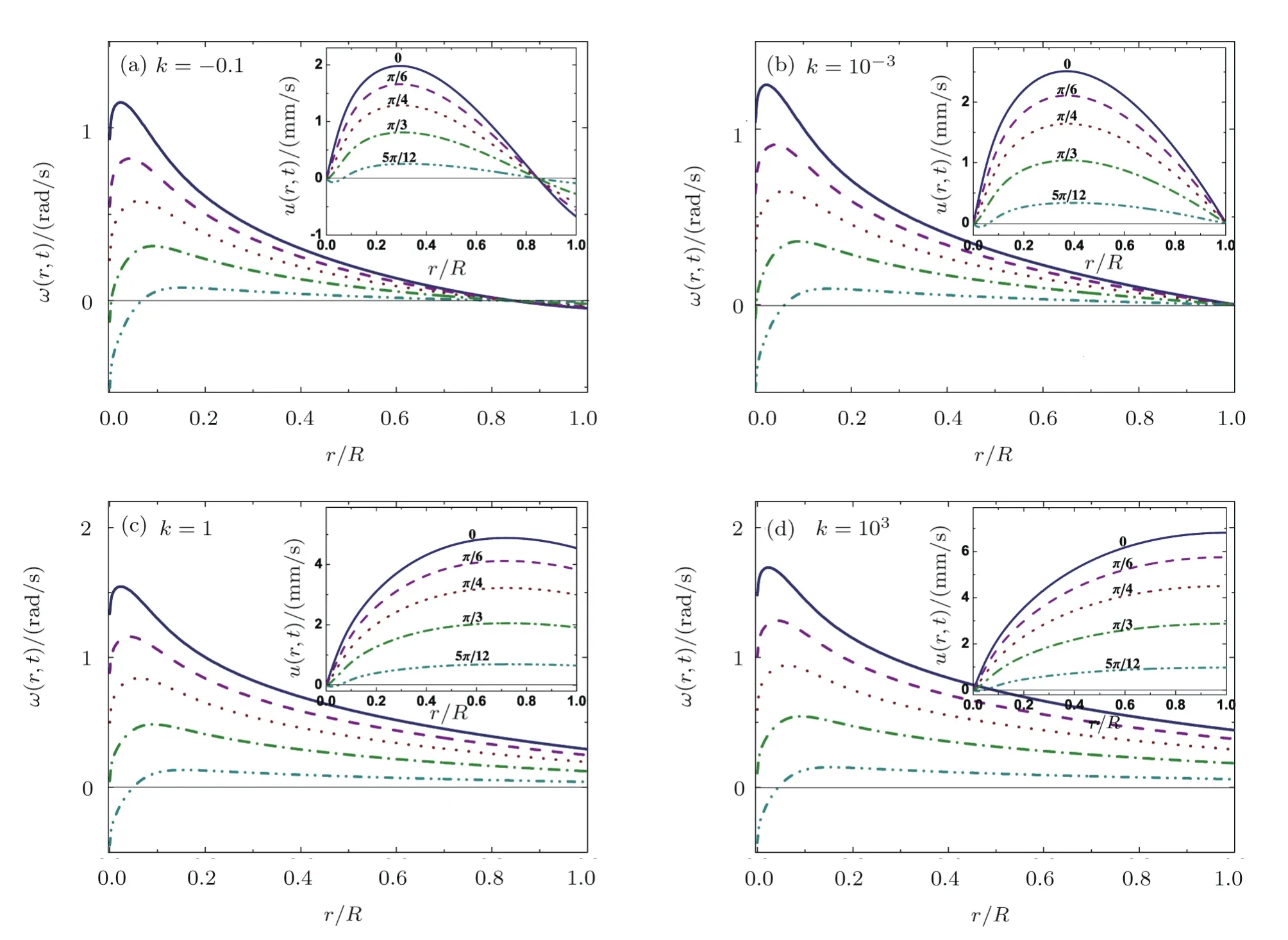
Fig.8 The profiles of the angular velocity of the rotating ACM with different k values for various values of φ(φ =0,π/6,π/4,π/3,5π/12)at time t=1000 s:(a)k= −0.1;(b)k=10−3;(c)k=1;(d)k=103.The insets show the profiles of the corresponding linear velocity of each figure.The frequencies of the AC fields are 0.5 Hz.As φ increases,the rotation speed not only decreases gradually,but also its maximum moves away from the center of the film.

4 Summary and Conclusions

We presented a new approach for studying effects of interfaces on polar liquids:we expounded their impact on the novel PLFMs’ fluid dynamics.By introducing slip boundary conditions in their DCM and ACM models,[11−12]we computed their EHD rotation velocity distributions and showed these agree with the existing experimental ones and those obtained with numerical techniques.Though the DCM and ACM models are yet rather simple and the only liquid parameters explicitly included are viscosity,density,dielectric permittivity and yield stress,the agreement signi fies PLFMs’potential for exploring effects of interfaces on polar liquids.

The EHD motions’high sensitivity to the boundary slip lengthls,which reflects the interface’s impact on the liquid,implies ILZs’physical properties are extractable by comparing calculated and measured speed distributions.The simplicity of our models evokes searching for straightforward relations between velocities’distributions,in particular their extremums,and ILZs’parameters is worthwhile.Identifying such relations,we expect to facilitate easy extraction of ILZs’parameters from observed PLFMs’velocity distributions.Our central results support this evocation:PLFMs’rotation speed distributions are independent of the absolute values of thelsand the liquid film’s radiusR,but are associated with their ratiok=ls/R;kdetermines the type of boundary slippage;kaffects PLFMs’linear and angular velocities magnitudes and location of their extremums.

With our study eliciting the strong dependence of the PLFMs’EHD motions onls,it also suggests improvements of our models:Replacinglsconstant value in Eq.(3)with a function expressinglsdependence on ILZ’s properties,computing speed distributions and comparing these with experimental data promise deeper understanding of interface effects.In particular,solid- fluid interactions,surface roughness,wettability,[41]the presence of gaseous layers[23,48]and dipole moment of polar liquids[49]effects onlsshould be assessed.In the special case of the ∼ 10−4m wide EZ adjacent to hydrophilic membranes or reactive metals,a relevant improvement in our model concernsµ,εandρ.Their values in the EZ are much higher than that of its adjacent liquid and depend on the distance from the interface,[2]therefore replacing their constant values in our model with functions depending onrpromises deeper understanding of EZ properties.

Our study also has important implications for the PLFM itself.As we predicted in a previous publication,[13]by applying different types of electrolysis and external electric fields(e.g.,square wave fields,variations in their frequency),PLFMs can operate as washers,centrifuges or mixers.Optimizing these devices requires knowledge on boundary effects on their EHD motions.For example,we expect largelsto accelerate PLFMs’mixing effects.

We conclude with noting our study is but a modest first step to employing PLFMs for unraveling ILZs’riddles on the one hand and optimizing the DCM’s and ACM’s technological performance on the other hand.With PLFMs’prospective contribution to solving ILZs’riddles and its far reaching implications,e.g.,understanding biological water(in living organisms water can be considered interfacial water,because it is but a fraction of a micron from a surface(cell membranes,macromolecules,etc.)),our study signi fies the study of PLFM’s have repercussions for basic science and technology far beyond those speci fied in Scienti fic American[50]reporting its invention: “Here’s a fun science project:Iranian researchers have found they can stir up a vortex in a thin film of water simply by applying an electric field. ···Although such a liquid motor is unlikely to power your car any time soon,they say it might be useful for mixing fluids for industrial applications or in studying turbulence in two dimensions”.

Appendix A Orthogonality Relations Among J1(λnξ)

The first differential equation in Eq.(6)may be simplified as

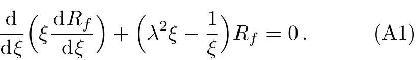
Ifm/=n,λm/=λn,insertingJ1(λnξ)andJ1(λmξ)into Eq.(A1),respectively,we obtain

LetJ1(λmξ)multiply Eq.(A2),J1(λnξ)multiply Eq.(A3),and the former minus the latter,then calculate the integral of them from 0 to 1,we obtain

Sinceλnandλmshould satisfy Eq.(7),we obtain

On inserting Eq.(A5)into Eq.(A4),one finds form/=n,

Next,let us discuss the casem=n.Whenm→n,i.e.,whenλm→λn,ifλnsatisfies the first equation in Eq.(A5),λmdoes not satisfy the second equation in Eq.(A5),i.e.,

Asm→n,from Eq.(A4)we have

Applying L Hospital rule to the right hand of Eq.(A7),i.e.,deducing the derivative of the numerator and denominator with respect toλm,respectively,we obtain

From Eq.(A2)and the first equation of Eq.(A5),we obtainInserting them into Eq.(A8),we obtain

Combining Eq.(A6)with Eq.(A9),we obtain the orthogonality relations given by Eq.(8).

Tamar Yinnon expresses her appreciation for Prof.A.M.Yinnon’s continuous support and encouragement.We express our gratitude to the referees for their constructive remarks.

[1]J.C.Henniker.Rev.Mod.Phys.21(1949)322.

[2]J.M.Zheng,W.C.Chin,E.Khijniak,E.Khijniak Jr.,and G.H.Pollack,Adv.Coll.Inter.Sci.23(2006)19;G.H.Pollack,Int.J.Des.Nat.Ecodyn.5(2010)27;B.Chai,H.Yoo,and G.H.Pollack,J.Phys.Chem.B 113(2009)13953;B.Chai and G.H.Pollack,J.Phys.Chem.B 114(2010)5371;B.Chai,J.M.Zheng,Q.Zhao,and G.H.Pollack,J.Phys.Chem.A 112(2008)2242;B.Chai and G.H.Pollack,J.Phys.Chem.B 114(2010)5371;B.Chai,A.G.Mahtani,and G.H.Pollack,Contemp.Mater.III-1(2012)1;B.Chai,A.G.Mahtani,and G.H.Pollack,Contemp.Mater.IV-1(2013)1;G.H.Pollack,The Fourth Phase of Water–Beyond Solid,Liquid,and Vapor,Ebner and Sons,Seattle(2013).

[3]R.Germano,E.Del Giudice,A.De Ninno,et al.,Key Eng.Mater.543(2013)455.

[4]T.A.Yinnon,V.Elia,E.Napoli,R.Germano,and Z.Q.Liu,Water 7(2016)96.

[5]A.Amjadi,R.Shirsavar,N.H.Radja,and M.R.Ejtehadi,Micro fluid.Nano fluid.6(2009)711.

[6]R.Shirsavar,A.Amjadi,A.Tonddast-Navaei,and M.R.Ejtehadi,Exp.Fluids 50(2011)419.

[7]R.Shirsavar,A.Amjadi,M.R.Ejtehadi,M.R.Mozaffari,and M.S.Feiz,Micro fluid.Nano fluid.13(2012)83.

[8]A.Amjadi,R.Nazi fi,R.M.Namin,and M.Mokhtarzadeh,arXiv:1305.1779v1(2013).

[9]M.S.Feiz,R.M.Namin,and A.Amjadi,Phys.Rev.E 92(2015)033002.

[10]A.Amjadi,M.S.Feiz,and R.M.Namin,Micro fluid.Nano fluid.18(2015)141.

[11]Z.Q.Liu,Y.J.Li,G.C.Zhang,and S.R.Jiang,Phys.Rev.E 83(2011)026303.

[12]Z.Q.Liu,G.C.Zhang,Y.J.Li,and S.R.Jiang,Phys.Rev.E 85(2012)036314.

[13]Z.Q.Liu,Y.J.Li,K.Y.Gan,S.R.Jiang,and G.C.Zhang,Micro fluid.Nano fluid.14(2013)319.

[14]Z.Q.Liu,K.Y.Gan,Y.J.Li,G.C.Zhang,and S.R.Jiang,Acta Phys.Sin.61(2012)134703(in Chinese).

[15]E.V.Shiryaeva,V.A.Vladimirov,and M.Y.Zhukov,Phys.Rev.E 80(2009)041603.

[16]F.P.Grosu and M.K.Bologa,Surf.Eng.Appl.Electrochem.46(2010)43.

[17]F.Q.Song and L.Yu,Adv.Mater.Res.594(2012)2684.

[18]J.F.Zhang and D.Y.Kwok,Phys.Rev.E 70(2004)056701.

[19]E.Lauga,M.P.Brenner,and H.A.Stone,inHandbook of Experimental Fluid Dynamics,Chapter 19,eds.C.Tropea,A.Yarin,J.F.Foss,Springer,Berlin(2007).

[20]P.Joseph,C.Cottin-Bizonne,J.M.Benoît,C.Ybert,C.Journet,P.Tabeling,and L.Bocquet,Phys.Rev.Lett.97(2006)156104.

[21]C.H.Choi and C.J.Kim,Phys.Rev.Lett.96(2006)066001.

[22]C.Lee,C.H.Choi,and C.J.Kim,Phys.Rev.Lett.101(2008)064501.

[23]E.Karatay,A.S.Haase,C.W.Visser,C.Sun,D.Lohse,P.A.Tsai,and R.G.Lammertink,Proc.Natl.Acad.Sci.U.S.A.110(2013)8422.

[24]Y.Wu,M.R.Cai,Z.Q.Li,X.W.Song,H.Y.Wang,X.W.Pei,and F.Zhou,J.Colloid Interface Sci.414(2014)9.

[25]E.D.Giudice,A.Tedeschi,G.Vitiello,and V.Voeikov,J.Phys.:Conf.Ser.442(2013)012028.

[26]A.A.Sonin,Freely Suspended Liquid Crystalline Films,John Wiley and Sons,New York(1998).

[27]S.Faetti,L.Fronzoni,and P.A.Rolla,J.Chem.Phys.79(1983)5054.

[28]S.W.Morris,J.R.de Bruyn,and A.D.May,Phys.Rev.Lett.65(1990)2378.

[29]Z.A.Daya,S.W.Morris,and J.R.de Bruyn,Phys.Rev.E 55(1997)2682.

[30]L.Bocquet and E.Charlaix,Chem.Soc.Rev.39(2010)1073.

[31]J.L.Barrat and L.Bocquet,Phys.Rev.Lett.82(1999)4671;J.Baudry,E.Charlaix,A.Tonck,and D.Mazuyer,Langmuir 17(2001)5232;D.C.Tretheway and C.D.Meinhart,Phys.Fluids 14(2002)L9;E.Lauga and M.P.Brenner,Phys.Rev.E 70(2004)26311;C.H.Choi and C.J.Kim,Phys.Rev.Lett.96(2006)066001;Y.Wu,M.R.Cai,Z.Q.Li,X.W.Song,H.Y.Wang,X.W.Pei,and F.Zhou,J.Colloid Interface Sci.414(2014)9.

[32]E.Del Giudice,G.Preparata,and G.Vitiello,Phys.Rev.Lett.61(1988)1085.

[33]S.Sivasubramanian,A.Widom,and Y.N.Srivastava,Physica A 345(2005)356;E.Del Giudice and G.Vitiello,Phys.Rev.A 74(2006)022105.

[34]G.Preparata,QED Coherence in Matter,World Scienti fic,Hong Kong(1995);G.Preparata,Phys.Rev.A 38(1988)233;R.Arani,I.Bono,E.Del Giudice,and G.Preparata,Int.J.Mod.Phys.B 9(1995)1813;E.Del Giudice and G.Preparata,A New QED Picture of Water,in Macroscopic Quantum Coherence,eds.E.Sassaroli,Y.N.Srivastava,J.Swain,and A.Widom,World Scienti fic,Singapore(1998);E.Del Giudice,J.Phys.:Conf.Ser.67(2007)012006;M.Buzzacchi,E.Del Giudice,and G.Preparata,Int.J.Mod.Phys.B 16(2002)3771;E.Del Giudice,A.Galimberti,L.Gamberale,and G.Preparat a,Mod.Phys.Lett.B 9(1995)953;E.Del Giudice,M.Fleischmann,G.Preparata,and G.Talpo,Bioelectromagn.23(2002)522;E.Del Giudice,G.Preparata,and M.Fleischmann,J.Elec.Chem.482(2000)110.

[35]S.Sivasubramanian,A.Widom,and Y.N.Srivastava,Physica A 301(2001)241;Int.J.Mod.Phys.B 15(2001)537;Mod.Phys.Lett.B 16(2002)1201;J.Phys.:Condens.Matter 15(2003)1109;C.Emary and T.Brandes,Phys.Rev.E 67(2003)066203;M.Apostol,Phys.Lett.A 373(2009)379.

[36]C.A.Yinnon and T.A.Yinnon,Mod.Phys.Lett.B 23(2009)1959;T.A.Yinnon and Z.Q.Liu,Water Journal 7(2015)19.

[37]C.Huang,et al.,Proc.Natl.Acad.Sci.USA 106(2009)15214.

[38]E.C.Fuchs,P.Baroni,B.Bitschnau,and L.Noirez,J.Phys.D 43(2010)105502.

[39]E.Del Giudice,E.C.Fuchs,and G.Vitiello,Water 2(2010)69.

[40]C.L.M.H.Navier,Mem.Acad.R.Sci.Inst.France 6(1827)839.

[41]C.Neto,D.R.Evans,E.Bonaccurso,H.J.Butt,and V.S.J.Craig,Rep.Prog.Phys.68(2005)2859.

[42]S.K.Ranjith,B.S.V.Patnaik,and S.Vedantam,Phys.Rev.E 87(2013)033303.

[43]F.Q.Song and L.Yu,Chinese Journal of Hydrodynamics A 28(2013)128.

[44]N.V.Priezjev,Phys.Rev.E 80(2009)031608.

[45]J.Mathews and R.L.Walker,Mathematical Methods of Physics,2nd ed.Addison-Wesley,New York(1971).

[46]Measured ILZs’properties indicate k’s physical lower bound is about−0.5:For PLFMs,typically 10−3m ＜R ＜ 10−2m.The maximal width of ILZs is of the order of 10−4m.Hence computed velocity distributions for−1＜ k＜ −0.5,though feasible with our model,are irrelevant.

[47]J.L.Xu and Y.X.Li,International Journal of Heat and Mass Transfer 50(2007)2571.

[48]O.I.Vinogradova and A.V.Belyaev,J.Phys.:Conden.Matter 23(2011)184104.

[49]J.H.J.Cho,B.M.Law,and F.Rieutord,Phys.Rev.Lett.92(2004)166102.

[50]http://www.scienti ficamerican.com/gallery/liquid-motor-revs-up/.