Construction and analysis of a new class of shape-preserving piecewise cubic polynomial curves
2018-01-08YANLanlanFANJiqiuCollegeofScienceEastChinaUniversityofTechnologyNanchang330013China
YAN Lanlan, FAN Jiqiu(College of Science, East China University of Technology, Nanchang 330013, China)
Construction and analysis of a new class of shape-preserving piecewise cubic polynomial curves
YAN Lanlan, FAN Jiqiu
(College of Science, East China University of Technology, Nanchang 330013, China)
This paper proposes a new class of shape-preserving piecewise cubic polynomial curves with both local and global shape control parameters. By presetting the properties of its basis functions and then solving equations, a set of polynomial basis functions with two shape parameters are derived, including the cubic uniform B-spline basis functions as a special case. Based on the relationship between the new basis functions and the cubic Bernstein basis functions, the totally positive property of the new basis functions is proved and a new class of piecewise cubic polynomial curves is therefore defined. The effect of the relative position of the control polygons’ side vectors onto the shape characteristic of the corresponding curve segments is analyzed. Necessary and sufficient conditions are obtained for the curve segments containing single or double inflection points, a loop or a cusp, or be locally or globally convex, which provide a theoretical guide for adjusting the shape of curve segments.
curve design; B-spline method; totally positive basis; shape parameter;shape analysis
保形分段三次多项式曲线的形状分析.浙江大学学报(理学版),2018,45(1): 044-053
Constructing practical basis functions to generate free-form curves and surfaces is an important topic in computer aided geometric design (CAGD).As a unified mathematical model with many desirable properties, B-splines, particularly the cubic B-splines, have gained widespread application in CAGD[1].Piecewise cubic B-spline curves with four consecutive control points for each curve segment is flexible and can be used conveniently.However, the positions of the cubic B-spline curves are fixed relatively to their control polygon.Although the weights in the cubic non-uniform rational B-spline curves possess an effect on adjusting the shape of the curves, how to change the weights to adjust the shape of a curve is sometimes quite opaque to the user.
To enhance the flexibility of B-spline models, some researchers have suggested many types of curves with shape parameters incorporated into the basis functions.For instance, XU et al[2]proposed three kinds of extensions of cubic uniform B-spline. The advantage of the extensions is that they have shape parameters, which can be used to adjust the shape of the curves without shifting the control points.COSTANTINI et al[3]presented a method for the construction of cubic like B-splines with multiple knots.The proposed B-splines are equipped with tension parameters, associated to the knots, which permit a modification of their shape.HAN[4]constructed piecewise quartic polynomial curves with a local shape parameter.HAN[5]defined piecewise quartic spline curves with three local shape parameters.HU et al[6]presented B-spline curves with two local shape parameters.ZHU et al[7]defined B-spline-like curves with two local shape parameters.
Totally positive property is one of the most important properties of basis functions.Although the schemes given in[2, 4-6] improved the control of the shape of B-spline curves, whether the basis functions have total positivity is unknown, so whether the curves have variation diminishing is unknown.Although the curves in[3,7] have variation diminishing, the basis functions are not cubic polynomials.For many applications in geometric modeling, it is often necessary to detect singularities and inflection points on curves, and convexity is important as an intuitive geometric concept as well.There are many publications[8-13]on this topic from different points of view.
This paper is aimed at constructing a cubic polynomial basis functions with total positivity.The associated curves have local control, adjustable shape, and have variation diminishing thus have a good shape control.Considering that a curve with variation diminishing is suitable for conformal design, we analyze the shape feature of the new curves.We give conditions on the existence of cusp, loop and inflection point.The results are summarized in a shape diagram like the one in[8, 10-11].Furthermore, the influence of the shape parameters on the shape diagram and their ability for adjusting the shape of the curves is discussed.
The rest of the paper is organized as follows.Section 1 gives the basis functions and their properties.Section 2 defines the curves and gives their properties.Section 3 analyzes the shape feature of the curve segments.Section 4 defines the surfaces.Section 5 concludes the paper.
1 Basis functions and their properties

(1)

Theαβbasis can be rewritten in Bernstein basis functions form, i.e.,
(b0(t),b1(t),b2(t),b3(t))=

(2)
where |Jij,kl| denotes the minor formed by thei,jrows andk,lcolumns ofJ.The matrixJhas 16 third-order minors as follows:
where |Jijk,lmn| denotes the minor formed by thei,j,krows andl,m,ncolumns ofJ.Besides,

(3)

Theorem1Theαβbasis has the following properties:
(a) Degeneracy: Whenα=-1,β=0, theαβbasis is the cubic uniform B-spline basis.
(c) Symmetry:bi(1-t)=b3-i(t)(i=0,1,2,3).
(d) Property at the endpoints: For arbitraryαandβ, we have
and forα=-1,β=0, we have

(f) Non-negativity:bi(t)≥0(i=0,1,2,3).
(g) Total positivity: Theαβbasis forms a normalized totally positive basis of the space Ω={1,t,t2,t3}.
ProofWe shall prove (e)and(g).The remaining can be easily obtained by formula (1) or (2).

(g) The cubic Bernstein basis is the normalized B-basis of the space Ω. Thus, by formula (2), lemma 1, and the properties (b)and (e), we know theαβbasis is a normalized totally positive basis.
2 The αβ curves and their properties
Definition2Given control pointsPi(i=0,1,…,n)∈R2orR3and knotsu1 i=1,2,…,n-2, i=1,2,…,n-2. Theorem2From the properties of theαβbasis, we can obtain the following properties of theαβcurves. (a) Affine invariance. (b) Symmetry: When taking the sameαβbasis, the two polygons,Pi-1,Pi,Pi+1,Pi+2andPi+2,Pi+1,Pi,Pi-1,describe the sameαβcurve segment; The only thing that changes is the direction of traversal of the parameter. (c) Local control: Changing one control point of anαβcurve, four segments will change mostly. (d) Endpoint property: For arbitraryαandβi, we have and forα=-1,βi=0, we have RemarkBy the endpoint property, we can see that the position of the starting and ending points of the curve segment only related to the parameterα. The valueβi-αdecides to the length of the tangent vector at the starting and ending points, thus decides to the degree of blending of theith curve segment. (e) Continuity: In general, theith and (i+1)thαβcurve segments areG1continuous at the junction, and they areG2continuous whenα=-1,βi=βi+1=0. (f) Shape adjustable: The parametersαandβican be used to adjust the shape of theαβcurve without changing the control points.Theαis a global parameter, whileβiis a local parameter.The change ofβiwill only change the shape of theith segment. (h) Variation diminishing and convexity-preserving. Fig.1 The open αβ curves Fig.2 The closed αβ curves As can be seen in figs.1 and 2, the shape ofαβcurves can reflect the shape of the control polygon well. We consider anαβcurve segment ai=Pi-Pi-1,i=1,2,3, thenp(t)can be rewritten as p(t)=P0+[1-b0(t)]a1+[b2(t)+ (4) We first consider the case ofa1not parallel toa3. Sincea1anda3are linearly independent,a2can be represented by the linear combination ofa1anda3.Without loss of generality, leta2=ua1+va3, and substitute it into formula (4), and then we have p(t)=P0+{1-b0(t)+u[b2(t)+b3(t)]}a1+ (5) The necessary condition that the curvep(t)has a cusp isp′(t)=0(0 Letp′(t)=0, fora1anda3are linearly independent, we obtain and then the following parametric curveC≜C(t)can be obtained. (6) To facilitate the analysis of the geometric properties ofC, we rewrite it in the form of quadratic rational Bézier curve, i.e, (7) (8) Let (u0,v0)∈C, and 0 p′(t)=p″(t0)(t-t0)+O(t-t0), we can see that the direction ofp′(t)is contravariant when it passes throught0.It shows thatCis the cusp curve, that is, the curvep(t)has cusp if and only if (u,v)∈C. The sufficient and necessary condition that the curvep(t)has a loop is that there exists 0≤t1 {b0(t2)-b0(t1)+u[b2(t1)+b3(t1)-b2(t2)- b3(t2)]}a1+{b3(t1)-b3(t2)+v[b2(t1)+ b3(t1)-b2(t2)-b3(t2)]}a3=0. Fora1anda3are linearly independent, we obtain (9) where (t1,t2)∈Δ={(t1,t2)∈R2|0≤t1 The parametric equations ofL1andL2are as follows: (10) (11) The curvesL1andL2can be rewritten in the form of quadratic rational Bézier curves (12) (13) (14) wheret∈(0,1). Eliminate the parametert, we obtain The binormal vector ofp(t)isγ(t)=p′(t)∧p″(t), wherep′(t)∧p″(t)is the wedge product ofp′(t)andp″(t). If the direction ofγ(t)is changed when it passes throught0, thenp(t0)(0 The binormal vectorγ(t)can be represented asγ(t)=f(t;u,v)(a1∧a3), where Sincea1×a3≠0,the direction ofγ(t)changes if and only if the sign off(t;u,v)changes.Hence, we only need to consider the sign change off(t;u,v). S= {(u,v)|uv<0}∪{(u,0)|-1 {(0,v)|-1 Dis the open region surrounded by the curveCand the coordinate axes. There is at least one straight linef(t0;u,v)=0 passing through every point (u0,v0)∈S∪D∪Ctangent to the curveC, heret0is the parameter corresponding to (u0,v0). From we can see that the sign off(t;u0,v0)does not change when it passes throught0. It meansp(t0)is not an inflection point, and there is no inflection point on the curvep(t). we can see that the sign off(t;u0,v0)changes when it passes throught0. It indicates thatp(t0)is an inflection point.Furthermore, there is only one straight line tangent to the curveCand passing through (u0,v0)∈S, the corresponding curvep(t)has a single inflection point.There are two straight lines tangent toCand passing through (u0,v0)∈D,the corresponding curvep(t)has double inflection points. We discuss the case of (u,v)∈N=R2(C∪S∪D∪L), see fig.3.At this point, there is no cusp or loop or inflection point on the curvep(t). And, the direction of the binormal vectorγ(t)does not change. Let From eq. (5), we obtain where (15) we can see that the sign ofφ(t;u0,v0)changes when it passes throught0. Sop(t)is local convex if (u,v)∈N1. we can see that the sign ofψ(t;u0,v0)changes when it passes throught0. Hence,p(t)is local convex if (u,v)∈N2. While if (u,v)∈N0=N(N1∪N2), the direction ofγ(t),m(t)andn(t)do not change, as a result the curvep(t)is global convex. Summarizing the discussion of section 3.1 to 3.4, we obtain the following conclusion. Theorem3Forαβcurve segment, letai=Pi-Pi-1,i=1,2,3, ifa1not parallel toa3anda2=ua1+va3,then the shape characteristic ofp(t)is totally determined by the distribution of the point (u,v)onuv-plane (see fig.3), i.e. Fig.3 gives the shape diagram of theαβcurve withα=-1,β=0. It is exactly the shape diagram of the traditional cubic uniform B-spline curve. Fig.3 The shape diagram of the αβ curve Examples of theαβapproximation curves with the six different shape characteristics are shown in fig.4.The settings of the parameters and the values of (u,v)are as follows: Fig.4 The αβ curves with different shape characteristics Ifa1parallel toa3, then after a similar discussion to section 3.1 to 3.4, we obtain the following conclusion. Theorem4Whena1‖a3, the curvep(t)has no singularity.If and only if the direction ofa1is the same as that ofa3, excluding the four control points collinear, the curvep(t)has one and only one inflection point. Changingαandβ, the shape diagram of theαβcurve will change accordingly, see fig.5.In fig.5, the settings of the parameters are as follows: Fig.5 The influence on shape diagram by α and β As can be seen from fig.5(a) to (c), with the increase ofα, the regionDreduces and the regionN0expands,while the regionSremains unchanged.As can be seen from fig.5(d) to (f), with the increase ofβ, the regionDreduces and the regionsN1,N2,Lexpand, while the regionsN0andSremain unchanged.In addition, from fig.5(d), we see that whenβ→α, the regionsN1,N2,Lreduce to zero.From fig.5(c), we see that whenα→0 andβ=0, the regionsN1,N2,LandDreduce to zero. From the above analysis, we can conclude that the regionScannot be changed by adjusting the shape parameters.That is to say, when there is only one inflection point on theαβapproximation curve, we cannot eliminate it by altering the values ofαandβ. However, when there is one cusp or one loop on the curve, or when the curve is local convex, it can be adjusted to a curve with two inflection points by takingβ→α. Further, the two inflection points can be removed by takingα→0 andβ=0. Meanwhile, the curve is adjusted to global convex. Definition3Given control pointsPij∈R3(i=0,1,…,m;j=0,1,…,n), two sets of knotsu1 wheres,t∈[0,1],i=1,2,…,m-2;j=1,2,…,n-2. All the patches constitute anαβsurface u∈[ui,ui+1],v∈[vj,vj+1], Theαβsurfaces have properties similar to theαβcurves.Fig.7 shows theαβsurfaces consisting of 7×4 patches defined by the same control net but different parameters.The settings of parameters are as follows: Fig.7 The αβ surfaces There are many extensions of cubic B-spline curves, but theαβcurves enjoy some advantageous properties from design.With variation diminishing and convexity-preserving, theαβcurves have a good shape control.Shape parameters are incorporated into theαβcurves, but we do not increase the degree of the basis polynomial, and therefore do not increase the amount of calculation.The shape diagram is useful for classifying and modifying the shape of theαβcurve.Notice that ifα=0, then theαβcurve segments interpolate to the two inner control points.Thus theαβcurves can be used to construct interpolation curves without solving equations.One of our future works is to discuss the shape parameter selection scheme of the interpolation curve. [1] FARIN G.CurvesandSurfacesforComputerAidedGeometricDesign[M]. San Diego: Academic Press,1993. [2] XU G, WANG G Z. Extended cubic uniform B-spline andα-B-spline[J].ActaAutomaticaSinica,2008,34(8): 980-984. [3] COSTANTINI P, KAKLIS P D, MANNI C. Polynomial cubic splines with tension properties[J].ComputerAidedGeometricDesign,2010,27(8): 592-610. [4] HAN X L. Piecewise quartic polynomial curves with a local shape parameter[J].JournalofComputationalandAppliedMathematics,2006,195(1-2): 34-45. [5] HAN X L. A class of general quartic spline curves with shape parameters[J].ComputerAidedGeometricDesign,2011,28(3): 151-163. [6] HU G, QIN X Q, JI X M, et al. The construction ofλμ-B-spline curves and its application to rotational surfaces[J].AppliedMathematicsandComputation,2015,266(C): 194-211. [7] ZHU Y P, HAN X L, LIU S J. Curve construction based on fourαβ-Bernstein-like basis functions[J].JournalofComputationalandAppliedMathematics,2015,273(1): 160-181. [8] HAN X L, HUANG X L, MA Y C. Shape analysis of cubic trigonometric Bezier curves with a shape parameter[J].AppliedMathematicsandComputation,2010,217(6): 2527-2533. [9] MONTERDE J. Singularities of rational Bezier curve[J].ComputerAidedGeometricDesign,2001,18(8): 805-816. [10] YANG Q M, WANG G Z. Inflection points and singularities on C-curves[J].ComputerAidedGeometricDesign,2004,21(2): 207-213. [12] LIU C Y.TheoryandApplicationofConvexCurvesandSurfacesinCAGD[D]. Enschede: University of Twente,2001. [13] YAN L L, YING Z W. Adjustable curves and surfaces with simple G3conditions[J].JournalofZhejiangUniversity:ScienceEdition,2016,43(1): 87-96. 严兰兰, 樊继秋 构造了一种保形并且形状可调的分段三次多项式曲线,并分析其形状特征与控制多边形之间的关系.首先,通过预设基函数的性质再解方程组,构造了一组带2个形状参数的多项式基函数,其包含三次均匀B样条基函数作为特例.然后,借助基函数与三次Bernstein基函数之间的关系证明了基函数的全正性,由这组基函数定义了一种分段三次多项式曲线,使该曲线拥有一个局部和一个全局形状参数.最后,分析了控制多边形边变量之间的相对位置关系对曲线段形状特征的影响,得到了曲线段拥有1个或2个拐点,1个二重点或1个尖点,为局部凸或全局凸时的充要条件.该结论为曲线段的形状调整提供了理论基础. 曲线设计; B样条方法; 全正基; 形状参数; 形状分析 TP 391 A 1008-9497(2018)01-044-10 date: April 5,2016. Supported by the NSFC(11261003, 11761008 ), the Natural Science Foundation of Jiangxi Province ( 20161BAB211028) and the Science Research Foundation of Jiangxi Province Education Department ( GJJ160558). AbouttheauthorYAN Lanlan (1982-),ORCID: http: //orcid.org/0000-0002-5472-9986, female, Ph.D,associate professor, the field of interest is CAGD, E-mail: yxh821011@aliyun.com. 10.3785/j.issn.1008-9497.2018.01.008


3 Shape analysis of the curve segment
b3(t)]a2+b3(t)a3.
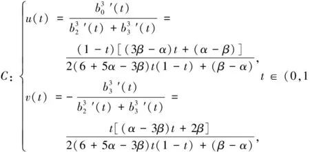
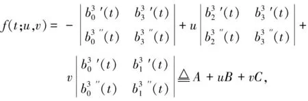
{b3(t)+v[b2(t)+b3(t)]}a3.3.1 The case of cusp


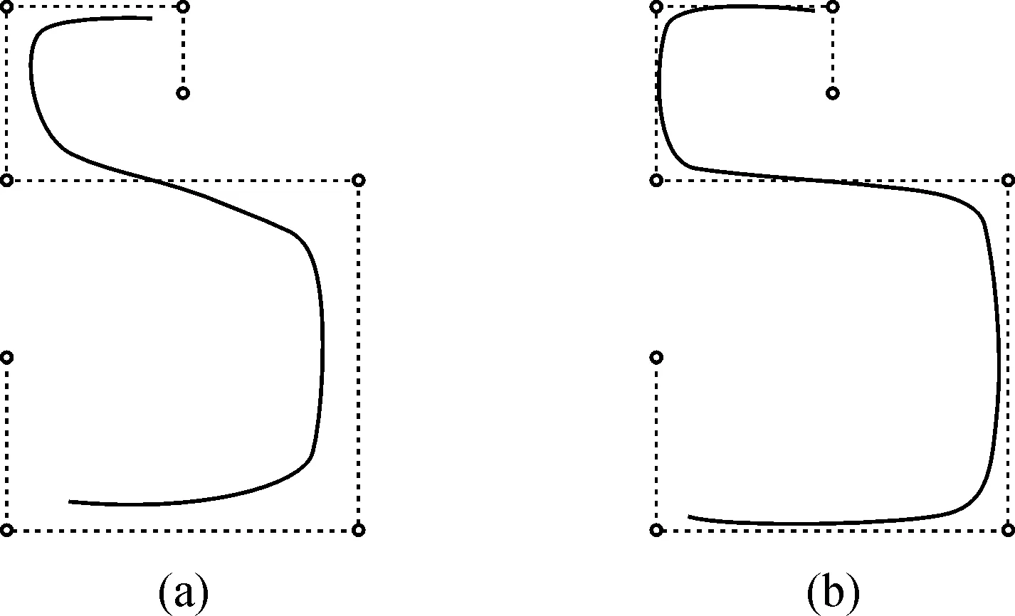
3.2 The case of loop


3.3 The case of inflection point


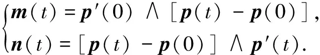
3.4 The case of convexity


3.5 Result


3.6 Regulatory effect of the shape parameters


4 The αβ surfaces


5 Conclusion
(东华理工大学 理学院, 江西 南昌 330013)