Calibration of three-axis magnetometer based on adaptive genetic algorithm
2017-09-12YUANGuangminYUANWeizhengLUODanyaoZHAOJingXUELiangLIXiaoying
YUAN Guang-min, YUAN Wei-zheng, LUO Dan-yao, ZHAO Jing, XUE Liang, LI Xiao-ying
(1. Ministry of Education Key Laboratory of Micro and Nano Systems for Aerospace, Northwestern Polytechnical University, Xi’an 710072, China; 2. Rocket Force University of Engineering, Xi’an 710025, China)
Calibration of three-axis magnetometer based on adaptive genetic algorithm
YUAN Guang-min1, YUAN Wei-zheng1, LUO Dan-yao1, ZHAO Jing1, XUE Liang2, LI Xiao-ying1
(1. Ministry of Education Key Laboratory of Micro and Nano Systems for Aerospace, Northwestern Polytechnical University, Xi’an 710072, China; 2. Rocket Force University of Engineering, Xi’an 710025, China)
In view that the precision of MEMS magnetometer can not meet the heading measurement requirement of the attitude measurement system, the error source of a three-axis magnetometer is modeled and analyzed, and a calibration method based on ellipsoid fitting and adaptive genetic algorithm is proposed. The adaptive genetic algorithm is employed to fit an ellipsoid using raw data obtained by the three-axis magnetometer, and the output data is corrected by using the ellipsoid estimated parameters to compensate offset, scale factors, hard iron and soft iron. The three-axis direction cosines of the sensor are fitted by least square method so that the calibration of the sensor can remove the non-orthogonality and mounting error. Finally, the proposed calibration method is applied to an attitude reference system to conduct the heading measuring experiments using raw data and calibrated data. Experiment results demonstrate that the heading deviation range is reduced to 0.7° from 4.5°,which shows that the heading accuracy is increased by 6.8 times.
MEMS magnetometer; calibration; ellipsoid fitting; adaptive genetic algorithm
MEMS three-axis magnetometer (TAM) is an important part of small aircraft’s attitude reference system. Due to the manufacture error, the commercial TAMs usually have such errors as offset, scale and nonorthogonality, etc.. This phenomenon leads to the error margin of about 1° - 2°[1-2]. In addition, the TAMs inevitably work under the influence of surrounding ferromagnetic materials, which badly affects the accuracy of navigation.
The common magnetometer calibration methods include multi-sensor fusing method[3], attitude-knowle-dge method[4], ellipse fitting method[5], ellipsoid fitting method[6], etc.. The multi-sensors fusing method fuses the data obtained from several sensors (TAM included)by using a filter, which relies on the reliabilities of other sensors. The attitude-knowledge method can only be used with the knowledge of attitude information, which requires using the navigation equipment with higher accuracy. The ellipse fitting method is simply in performing,which is only applied to plane motion. The ellipsoid fitting method is a novel calibration method, which simplifies the error model as an expression of an ellipsoid,and is allowed for simple implementation when the calibration accuracy is given.
A genetic algorithm, as a search algorithm, not only suits for complicate non-linear optimization but also keeps efficient in least-squares ellipsoid fitting. An SGA(Standard genetic algorithm) works in a random and direct way, however, it is easy to get stuck in local optimum. An AGA (adaptive genetic algorithm) is an improved GA, which tunes the genetic operators adaptively. Therefore, it can not only decrease the number of generations for the computational convergence, but also avoid getting stuck in local optimum. In this paper, we propose an ellipsoid fitting algorithm based on AGA to improve the heading measurement accuracy, and validate it by the test results.
1 Error sources analysis and error model of TAM
Considering the inevitable error, it is necessary to analyze the error source for the accurate calibration of TAMs. Generally, these errors are divided into three categories[7-8]: sensors error, mounting error and magnet error. The sensor errors include scale factors, offset and non-orthogonality. The magnet errors mainly include ferromagnetic materials (specifically refers to hard iron and soft iron, which distort the magnetic field detected by TAMs). The hard iron and soft iron are paramount interferences to TAM, in which the hard iron makes a shift, and the soft iron makes deformation and rotation on the detected magnetic field.
A mathematical model of TAM readings including the error sources is developed as follow:

Where Siis the matrix of the mounting error, N is the matrix of the nonorthogonality, Smis the matrix of the soft iron, Scis the vector of the scale factors, H is the vector of the hard iron, B is the offset vector, M is the geomagnetic vector, andis the measurement vector.
Considering the interaction between these errors and their combining interference to TAMs, it is impossible to make a separate error analysis on any part in the formula. According to ellipsoid fitting method[9-10], a conversion of Eq.(1) is given by Eq.(2):

Where A is the matrix combining mounting error and nonorthogonality, K is the matrix combining soft iron and scale factors, and P is the matrix combining hard iron and offset.
2 Ellipsoid model
In the axis-orthogonal case, the relation between M andMˆis shown as follows:

Expressing the variables K and P with 9 unknown variables in Eq.(6) as follows:
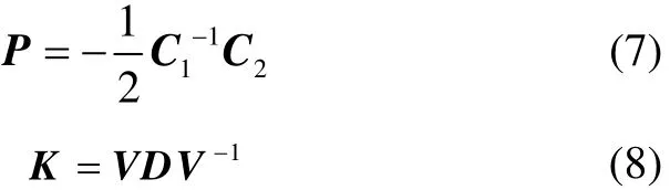
Where D=diag(d1d2d3)is diagonal matrix whose elements are the square roots of eigenvalues of C1, and V is the matrix composed by eigenvectors of C1.
First, fit an ellipsoid to raw data obtained by a TAM. Determine a solution of parameters of the ellipsoid shown in Eq.(6). Next determine matrix K and P by Eq.(7) and Eq.(8). Finally compensate the outputs by Eq.(9). So the calibrated measurements of the earth’s magnetic field are obtained.

Where M′is a corrected vector.
3 Misalignment model
Next, the mathematics model of the nonorthogonality and the mounting error is developed. As shown in Fig.1, the solid lines denote the axis of the global reference frame/earth-fixed coordinate system. The dotted lines denote the actual axis of the sensor reference frame.The angles between z-axis in global reference frame and 3 axes in the sensor frame are represented as α, β and γ respectively. When the sensor frame rotates around z-axis in the global frame, the TAM’s measurements are given by:


Fig.1 Nonorthogonality and mounting error of three-axis magnetometer
Eq.(10) is linear since α, β, and γ are constant.Therefore, the least-squares method can be employed to estimate cosα, cosβ, and cosγ.

Rxand Rycan be determined in the same way. So that A is gotten according to Eq.(12). The readings of TAM can be corrected using Eq.(13).


4 Parameters’ optimal solution of TAM error model
Genetic algorithms (GA) are intelligent algorithms that mimic the process of natural selection, which are especially suit for multi-parameter optimization. We design an AGA for least-square ellipsoid fitting. In GAs,it is essential to tune Pm(mutation probability) and Pc(crossover probability). High recombination rate would lead to premature convergence of the genetic algorithms.On the contrary, small mutation rate may lead to genetic drift. Too high mutation rate may result in losing the appropriate solution unless an elitist selection is employed.Therefore, the algorithm evaluates every individual in each generation by fitness in order to make a comparison with the relative average value. Then, it tunes Pmand Pcusing Eq.(14) and (15) to ensure the solution’s globality.Where fmaxis the maximal fitness value of the population, fminis the minimal fitness value of the population,faveis the average fitness value of the population, f′is the larger fitness value of two individuals to crossover,and f is the fitness value of an individual.

The selection mechanism is based on the relationship between the individual fitness and the average value.The individuals with bigger fitness are subjected to greater Pcand Pm, which means they will be protected soon.Conversely, the individuals with smaller fitness are subjected to smaller Pcand Pmand will be eliminated.
The chromosome of an individual (or a solution)represents the parameters of the ellipsoid fitted to be estimated. A chromosome contains 5 decimal bits. For any parameter, its estimating precision is (Xmax-Xmin)/105.After the global optimal solution is found, the parameters need to be decoded from the encoded solution.
Overall operation of the AGA is presented in Fig.2.

Fig.2 Flow chart of the adaptive genetic algorithm’s overall operation
First, an initial population of 180 individuals is created randomly. Next, the measurements are corrected using Eq.(9), where the variables are decoded from a solution. The fitness of the solution is evaluated using Eq.(16). And the half of individuals with higher fitness from the population is selected as the parent generation.

Where Miis the calibrated measurement vectors, and M0is geomagnetic vector.
Then, we pick two individuals from parent generation and check whether these two variables cross through Pc(Eq.(14)). Two-point technique is employed to perform crossover. We pick one individual from parent generation and check whether this one is mutated through Pc(Eq.(15)). And uniform-type technique is employed to perform mutation. Repeating the above process with generations in the evolution, and when the difference between the average fitness value of a certain generation and the elitist individual in this generation is small enough, the required precision of the solution is met. The algorithm stops when the difference between the average fitness and optimal fitness can be ignored (judged by Eq.(17)) because we suppose that the precision is same as expected at this moment. Finally, terminate the running of procedure. The global optimal parameters can be decoded from the individual of the highest fitness.

5 Test results and analysis
We employ an attitude reference system (an IMU and a TAM) to determine heading angles by using data acquired by the TAM before and after calibration. First,we hold the sensor and rotate it in all directions arbitrarily to acquire the data under different attitudes.Next, we employ the algorithm to fit an ellipsoid and estimate parameters, and plot a comparing figure of raw data and fitted ellipsoid.
As shown in Fig.3, each raw data point lies nearly on the surface of the fitted ellipsoid, which means that the ellipsoid is well-fitted. And K and P are determined by using Eq.(7) and Eq.(8).
Then, we level a rotating stage and align the system’s x-, y- and z-axis to vertical upward direction respectively.We rotate the stage and acquire the output data by the system, so that A can be determined by Eq.(11). The raw data can be corrected by Eq.(9) and Eq.(13).

Fig.3 Raw data and fitted ellipsoid
As shown in Fig.4, the ellipsoid where the thin gray broken lines lies in represents the ellipsoid fitted to the raw data. The thick gray line on the bottom half denotes the circle composed of the raw data in z-axis vertical upward rotation situation. The thin black solid lines depict the sphere fitted to the corrected data. And the thick black line on the sphere denotes the circle composed by the corrected data acquired in plane rotating.Note that the ellipsoid is clearly shifted and stretched in the z-axis and its maximum is clearly greater than the value of the earth’s magnetic field strength (524 nT). But the sphere is almost centered and its radius is approximately equal to the strength of the earth’s magnetic field.The plane where the thick gray line lies in is clearly not parallel to x-y plane, and is also not orthogonal to z-axis.However, the plane where the thick black line lies in is almost orthogonal to z-axis. Fig.4 shows that, after the calibration procedure, the positions, directions and magnitudes of the measurement vectors are all well corrected.
Finally, we post the TAM on the stage aligned to the global frame and make it rotate 1 circle with the same intervals of 45° and make a list about the heading information before and after the calibration, as shown in Tab.1.

Fig.4 Data before and after calibration
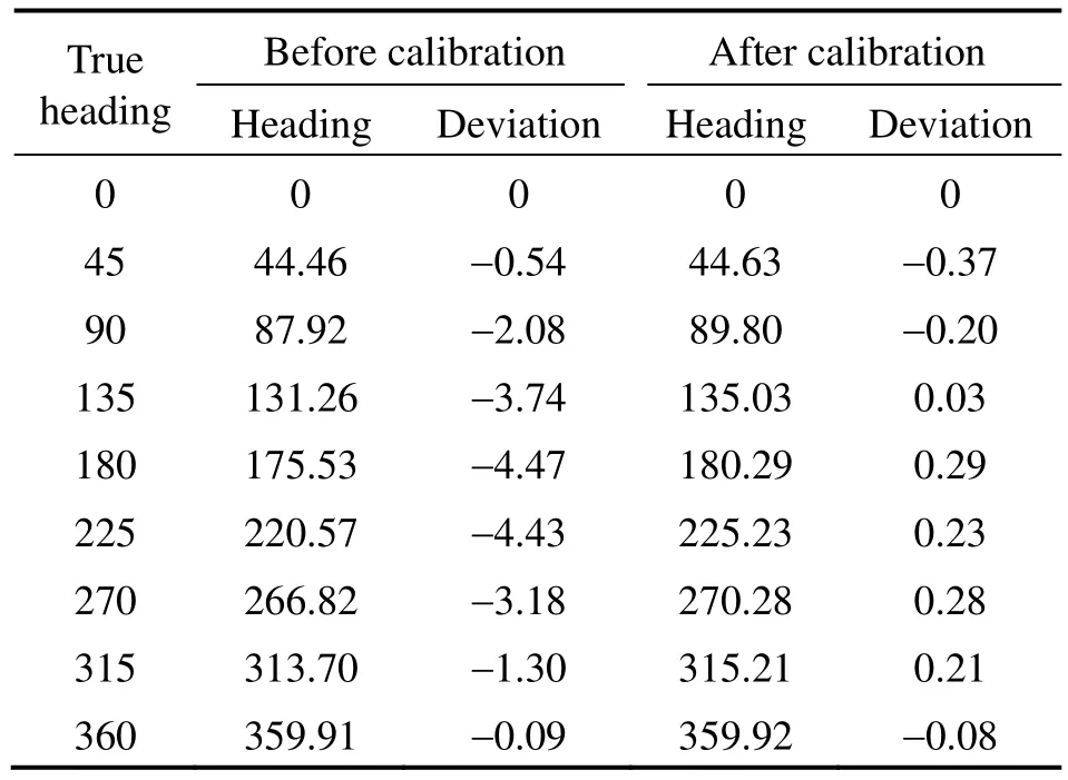
Tab.1 Heading information before and after calibration (°)
After calibration, the value of heading deviation range is reduced to 0.7° from 4.5°, as noted in the Tab.1.It demonstrates that the heading deviation by the proposed calibration procedure is decreased by approximately 6 times.
6 Conclusion
In summary, by analyzing the error source of TAM,we have established the error model and determined the relative calibration parameters. Moreover, a complete calibration procedure for TAMs is proposed and applied into an attitude reference system for calibrating the heading. The test result shows that the heading accuracy of the attitude reference system is significantly improved.The method has reference value for the application of TAMs in navigation system.
[1] Zhang Qi, Pang Hong-feng, Wan Cheng-biao. Magnetic interference compensation method for geomagnetic field vector measurement[J]. Measurement, 2016, 91: 628-633.
[2] Li Xiang, Li Zhi. A new calibration method for tri-axial field sensors in strap-down navigation systems[J]. Measurement Science and Technology, 2012, 23(10): 2852- 2855.
[3] Liu T, Inoue Y, Shibata K. A simplified magnetometer calibration method to improve the accuracy of threedimensional orientation measurement[J]. ICIC Express Letters, 2012, 6(2): 523-528.
[4] Fang Jian-cheng, Sun Hong-wei, Cao Juan-juan, et al. A novel calibration method of magnetic compass based on ellipsoid fitting[J]. IEEE Transactions on Instrumentation and Measurement, 2011, 60(6): 2053-2061.
[5] Yuan Guang-min, Yuan Wei-zheng, Qin Wei, et al. Research on magnetic heading error compensation technology under the strong magnetic interference[J]. Advances in Aeronautical Science and Engineering, 2012(2): 218-222.
[6] Bonnet S, Bassompierre C, Godin C, et al. Calibration methods for inertial and magnetic sensors[J]. Sensors and Actuators a-Physical, 2009, 156(2): 302-311.
[7] Olivares A, Ruiz-Garcia G, Olivares G, et al. Automatic determination of validity of input data used in ellipsoid fitting MARG calibration algorithms[J]. Sensors, 2013,13(9): 11797-11817.
[8] Zhang Qi, Li Ji, Chen Di-xiang, et al. Method and experiment for compensating the interferential magnetic field in underwater vehicle[J]. Measurement, 2014, 47(1): 651-657.
[9] Liu Guang-sheng, Guan Zhen-zhen. Research of interference field measurement and error compensation for geomagnetic navigation[J]. Applied Mechanics and Materials,2014, 602-605: 1586-1589.
[10] Foster C C, Elkaim G H. Extension of a two-step calibration methodology to include nonorthogonal sensor axes[J].IEEE Transactions on Aerospace and Electronic Systems,2008, 44(3): 1070-1078.
基于自适应遗传算法的三轴磁强计校准
袁广民1,苑伟政1,罗丹瑶1,赵 婧1,薛 亮2,李晓莹1
(1. 西北工业大学 空天微纳系统教育部重点实验室,西安 710072;2. 火箭军工程大学,西安 710025)
针对MEMS磁强计的精度无法满足姿态测量系统的航向角测量要求,对磁强计的误差来源进行了模型化分析,设计了一种基于自适应遗传算法的空间椭球磁强计校准方法。首先,采取自适应遗传算法,对磁强计测量的原始数据进行空间椭球的拟合,用估计的参数进行刻度系数、软磁干扰、硬磁干扰与零位偏置的综合误差补偿。其次,利用最小二乘法求解出非正交轴的方向余弦,进行非正交误差和安装误差的补偿。最后,将该方法应用到某姿态测量系统中,分别用未补偿和补偿后的数据进行姿态测量实验,实验结果表明该方法准确计算出磁强计的误差参数,使补偿后的航向角精度提高了6.8倍。
MEMS磁强计;校准;椭球拟合;自适应遗传算法
U666.1
:A
1005-6734(2017)03-0382-05
(References):
2017-02-01;
:2017-05-20
航空基金(20160553004);111引智基地(B13044);国家自然科学基金(61503390);陕西省自然科学基金(2016JQ6014)
袁广民(1977—),男,博士研究生在读,副研究员。E-mail: yuangm@nwpu.edu.cn
联 系 人:李晓莹(1969—),女,副教授。E-mail: xiaoy@nwpu.edu.cn
10.13695/j.cnki.12-1222/o3.2017.03.019