Symmetrization for Fractional Elliptic and Parabolic Equations and an Isoperimetric Application∗
2017-07-02YannickSIREJuanLuisZQUEZBrunoVOLZONE
Yannick SIRE Juan Luis VÁZQUEZ Bruno VOLZONE
(Dedicated to Haim Brezis,great master of analysis,on his 70th birthday)
1 Introduction
In this paper,we develop further the theory of symmetrization for fractional Laplacian operators initiated in[25,64–65],both in the elliptic and the parabolic setting,by extending it to a natural version of the fractional Laplacian defined on a bounded domainΩof RNwhich is known as the restricted fractional Laplacian.This research direction combines classical themes in the study of nonlinear elliptic and parabolic equations,like symmetrization and accretive operators,with the recent interest in nonlocal versions of the diffusion operators,specially the fractional Laplacians.As an application of the obtained comparison results,we derive an original proof of the Faber-Krahn inequality(FKI for short)for such operators defined on the bounded domainΩ.
Before entering into the description of our results,we review in this introduction the necessary information about symmetrization,the elliptic-to-parabolic technique used to generate evolution semigroups,the precise definition of the fractional Laplacian operators and the relation among these topics.This constitutes a sort of review part of this paper.
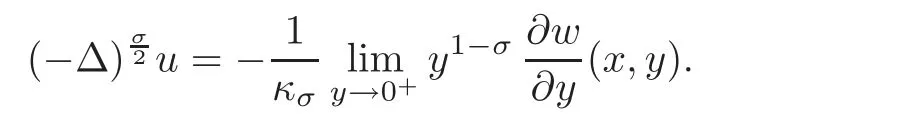
Definitions of fractional Laplacians on bounded domainsWhen working in the whole space domain RN,there are several equivalent definitions of the fractional Laplacian operatorclassical references being[39,53].The interest in these operators has a long history in probability since the fractional Laplacian operators of the formare infinitesimal generators of stable Lévy processes(see[1,7,57]).Further motivation and references on the literature are given for instance in[11,64].A particular definition that was convenient for symmetrization purposes defines the operator for every given 0<σ<2 as the trace of a suitable Dirichlet-Neumann problem via an extended potential function w that solves an elliptic equation in an upper half-space in H+=RN×(0,∞)⊂ RN+1.This is usually called Caff are lli-Silvestre extension(see[18]).It allows to reduce nonlocal problems involvingto suitable local problems(actually,a degenerate-singular elliptic equation),defined in one more space dimension.
When we work on a bounded domainΩ⊂RN,things get complicated because there are several options for defining the fractional Laplacian operatorTwo of them appear often in the recent literature.In our previous work[65]on symmetrization,we followed one of these approaches to define the fractional Laplacian as the Dirichlet-to-Neumann map,through an extended potential function defined in a cylinder C=Ω×(0,∞)⊂RN+1,as was proposed in[17,22].Zero values are assigned on the lateral boundary of C.We call this operator the spectral version of the fractional Laplacian onΩ.Let us call this operator L1(L stands for the Laplacian).This setting allowed us to derive in[65]the desired symmetrization results,which extend the standard symmetrization theory applied to elliptic and parabolic equations driven by the standard Laplacian operator.But let us recall that there are remarkable restrictions on their validity in the form of conditions on the nonlinearities that are allowed in the equations.
In this paper,we take the second usual approach to definewhich seems to be more natural in many applications.It consists in keeping the definition of fractional Laplacian in RNbut asking it to act on the null-extensions to RNof functions u(x)defined inΩ.So in principle,we can use the most common formulation with a hyper-singular kernel
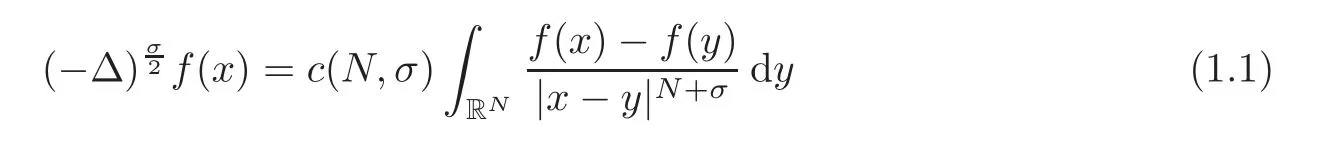
on the condition that f(y)=0 for y?∈ Ω.Let us call this operator L2.This option was called the restricted Laplacian on a bounded domain(see[49,10]),but we prefer the name natural fractional Laplacian with Dirichlet conditions in this paper.The discussion on the relations and differences between the two types of operators on bounded domains is currently being investigated by several authors.Thus,Musina and Nazarov[44]used the name fractional Laplacian with Navier conditions for the spectral version,and fractional Laplacian with Dirichlet conditions for the restricted version.
Here,we want to extend to operator L2the symmetrization theory we had developed for L1in[25,64].This has an independent interest since there are subtle differences between the two operators(see[10,12]).
SymmetrizationSymmetrization is a very ancient geometrical idea that is used nowadays as an efficient tool of obtaining a prioriestimates for the solutions of different partial differential equations,notably those of elliptic and parabolic type.Since the topic is so well-known,let us only recall some facts that are relevant here.Symmetrization techniques appear in classical works like[34,47].The application of Schwarz symmetrization to obtaining a priori estimates for elliptic problems was already described in[42,66].The standard elliptic result refers to the solutions of an equation of the form

posed in a bounded domainΩ⊆RN;the coefficients{aij}are assumed to be bounded,measurable and satisfy the usual ellipticity condition;finally,we take zero Dirichlet boundary conditions on the boundary ∂Ω.The classical analysis introduced by Talenti[54–55]leads to pointwise comparison between the symmetrized version(more precisely the spherical decreasing rearrangement)of the actual solution of the problem u(x)and the radially symmetric solution v(|x|)of some radially symmetric model problem which is posed in a ball with the same volume asΩ.Sharp a priori estimates for the solutions are then derived.Extensions of this method to more general problems or related equations led to a copious literature.
Elliptic approach to parabolic problemsFor parabolic problems,this pointwise comparison fails and the appropriate concept is comparison of concentrations(see[2–3,58]).The latter considers the evolution problems of the form

where A is a monotone increasing real function,and u0is a suitably given initial datum which is assumed to be integrable.For simplicity,the problem was posed for x∈RN,but bounded open sets can be used as spatial domains.The novel idea of the paper is to use the famous Crandall-Liggett Implicit Discretization theorem(see[24])to reduce the evolution problem to a sequence of nonlinear elliptic problems of the iterative form

where tk=kh,and h>0 is the time step per iteration.Writing A(u)=v,the resulting chain of elliptic problems can be written in the common form

General theory of these equations(see[8]),ensures that the solution map

is a contraction in some Banach space,which happens to be L1(Ω).Note that the constant h>0 is not essential,it can be put to 1 by scaling.In that context,the symmetrization result can be split into two results:
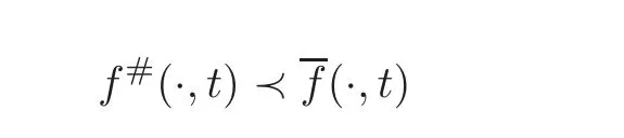
(i)The first one applies to rearranged right-hand sides and solutions.It says that if two r.h.s.functions f1,f2,are rearranged and satisfy a concentration comparison of the formthen the same applies to the solutions,in the form.1For the definition of the order relation≺,see Section 7.
(ii)The second result aims at comparing the solution v of(1.4)with a non-rearranged function f with the solutioncorresponding to f#,the radially decreasing rearrangement of f.We obtain thatis a rearranged function andis less concentrated than
This precise pair of comparison results can be combined to obtain similar results along the whole chain of iterations u(tk)of the evolution process,if discretized as indicated above.This allows in turn to conclude the symmetrization theorems(concentration comparison and comparison of Lpnorms)for the evolution problem(1.2).This approach can be used in many different situations.In particular,it will be used below.
Symmetrization for equations with fractional operatorsThe study of elliptic and parabolic equations involving nonlocal operators,usually of fractional type,is currently the subject of great attention.Symmetrization techniques were first applied to PDEs involving fractional Laplacian operators in[25],where the following linear elliptic case is studied:

This paper uses an interesting technique of Steiner symmetrization of the extended problem,based on the Caffarelli-Silvestre extension for the definition ofσ-Laplacian operator.In[64]the last two authors of the present paper were able to improve on that progress and combine it with the parabolic ideas of[58]to establish the relevant comparison theorems based on symmetrization for linear and nonlinear parabolic equations.To be specific,they dealt with equations of the form

Following the known theory for the standard Laplacian,the nonlinearity A is an increasing real function such that A(0)=0,and we accept some extra regularity conditions as needed,like A smooth with A?(u)>0 for all u>0.The problem is posed in the whole space RN.Special attention is paid to cases of the form A(u)=umwith m>0;the equation is then called the fractional heat equation(FHE for short)when m=1,the fractional porous medium equation(FPME for short)if m>1,and the fractional fast diffusion equation(FFDE for short)if m<1.Let us recall that the linear equationis a model of so-called anomalous diffusion,a much studied topic in physics.
The results of[25,64]include a comparison of concentrations,in the formthat parallels the result that holds in the standard Laplacian case;note however that no pointwise comparison is obtained,so the result looks a bit like the parabolic results of the standard theory mentioned above.[64]considered both problems posed in the whole space and on a bounded domain.In the latter case,the spectral fractional Laplacian is always chosen.
2 Outline of Results of the Present Pap er
We are interested in considering the application of such symmetrization techniques to linear or nonlinear elliptic and parabolic equations with fractional Laplacian operators posed on a bounded domain,when the natural(i.e.,restricted)version of fractional Laplacian is used.We denote the operator by L2.
Parabolic equationsTo be specific,we want to treat evolution equations of the form

We want to consider as nonlinearity A an increasing real function such that A(0)=0,and we may accept some other regularity conditions as needed,like A smooth with A?(u)>0 for all u>0.The problem is posed inΩ,a bounded subset of RNwith smooth boundary.The parabolic result is developed in Section 5 and has to be compared with the results of papers[64–65].We focus on the linear case A(u)=cu.This is the case that is needed in the isoperimetric application that we study in Section 6.
Elliptic equationsThe application of the method of implicit time discretization leads to the nonlinear equation of elliptic type

posed again in the whole spaceΩ⊂RNwith zero Dirichlet boundary conditions;h>0 is a non-essential constant,and the nonlinearity B is the inverse function to the monotone function A that appears in the parabolic equation(1.6).The elliptic results are developed in Sections 3–4 and have to be compared with the results of[25,64]where the equation is posed either in RNor inΩwith operator L1.Note that the elliptic results we get cover the standard linear case where the term B(v)disappears,and we set h=1.
A geometrical application(the Faber-Krahn inequality)As an application,we use the symmetrization results to prove the Faber Krahn inequality for the fractional Laplacian operator on a bounded domain in both versions considered above.We recall that the FKI is a classical eigenvalue inequality,due separately to[31,38],based on a conjecture by Rayleigh in 1877,that can be stated as follows.
LetΩbe a bounded domain in RN,and let B be the ball centered at the origin with Vol(Ω)=Vol(B).Let λ1(Ω)be the first eigenvalue of the Laplacian operator,with zero Dirichlet boundary conditions.Then λ1(Ω)≥ λ1(B),with equality if and only ifΩ =B almost everywhere.
Remark 2.1Note that we do not assume any regularity on the bounded domainΩbesides its openness.
This is a classical result in the calculus of variations and proofs can be found in the classical books like[20](see a recent proof in[15]).The question we want to address here is the following:Will the result also hold for the usual versions of the fractional Laplacian operatordefined on bounded domains of RNwith zero Dirichlet boundary conditions?
The answer is immediate in the case of the so-called spectral version of the Dirichlet fractional Laplacian,L1,since its eigenvalues,λk(L1;Ω),are directly related to those of the standard Laplacian,λk((−Δ);Ω),by the following formula:

However,no simple relation like this one happens for the natural fractional Laplacian with the definition restricted type,L2.
In Section 6,we use our comparison results to present an original derivation of the fractional FKI.It does not make use of any variational interpretation,but only of some properties of the evolution process.The FKI can also be studied either by probabilistic or variational methods.For completeness,we also present a variational derivation,see more details in the mentioned section.This latter proof is based on the original argument for the FKI for the Laplacian operator and relies on Pólya-Szegö inequalities.
Preliminary material and notationIn this paper,we use standard concepts and notations on symmetrization as fixed in[64].We gather the main facts that we did not present here in the first appendix for the reader’s convenience.
3 Elliptic Problem with Lower-Order Term
The case of the natural fractional Laplacian L2occupies our attention in this paper.We start our analysis by the following nonlocal elliptic problem with Dirichlet condition:
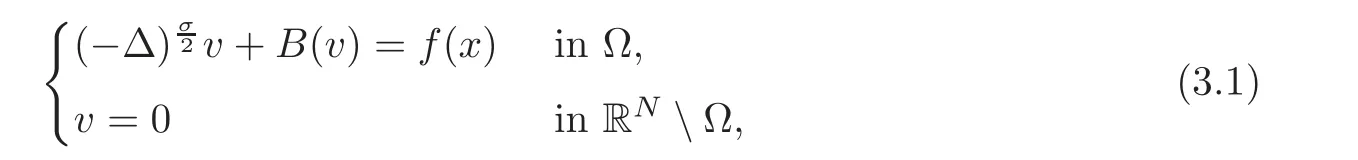
whereΩis an open bounded set of RN,σ∈(0,2),and f is an integrable function defined in Ω.We are interested in treating the case of a bounded domainΩ with the natural version of the fractional Laplacian.Exceptionally,Ωmay be RN,but this case was treated in[64].We assume that the nonlinearity is given by a functionwhich is smooth and monotone increasing with B(0)=0 and B?(v)>0.It is not essential to consider negative values for our main results,but the general theory can be done in that greater generality,just by assuming that B is extended to a function B:R−→ R−by symmetry,B(−v)= −B(v).Note that we have changed a bit the notation with respect to(2.2)in the introduction,by eliminating the constant h>0,but the change is inessential for the comparison results.
For simplicity,all the restrictions of the fractional Laplacian operator will be denoted byThe underlying assumption is that such operator will be restricted to the ground domain of each boundary value problem where it is involved.
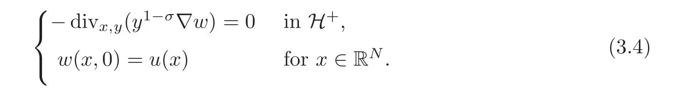
The extension methodThe Caffarelli-Silvestre method can be kept as extension to the whole H+,with the following important proviso:The extension must act on the null-extensions to RNof functions defined inΩ.In view of this discussion,a solution to(2.2)is defined here as the trace of a properly defined Dirichlet-Neumann problem in the following way:
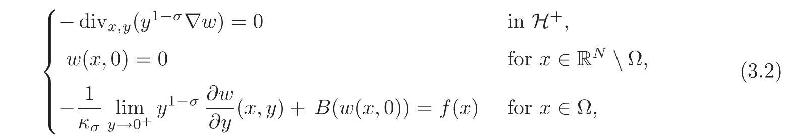
where
and κσis the constant(see[18]),but such a value is not important here.
3.1 Review of existence,uniqueness and main properties
If(3.2)issolved in an appropriate sense,then the trace of w over Ω,TrΩ(w)=w(·,0)=:v is said to be a solution to(3.1).Note that the trace of w on the bottom hyperplane{y=0}is the extension?v of the function v defined inΩby assigning the value zero outside ofΩ.This is what makes the difference with the case of the spectral Laplacian,where on the contrary the domain of the extended function w is the cylinder C=Ω×(0,∞)and w takes zero boundary conditions on the lateral boundary,Σ =∂Ω×[0,∞)(see[64]).In accordance with our choice of operator and in view of the iteration process that leads to the solution of the parabolic equations,we need only consider functions f that are restrictions toΩof functions defined in the whole of RN.
In order to make this more precise,we introduce the concept of weak solution to problem(3.2).It is convenient to define the weighted energy space

equipped with the norm

For an open set E of RN,we denote bythe classical fractional Sobolev space of orderover E.We recall that for anythere exists a uniqueσ-harmonic extensionof u to the half space H+,namely w solves
Then we write w=ExtH+(u).Moreover,for suitable functions u,we have
Now,in order to give a proper meaning of solution to a problem like(3.2)in a bounded domainΩ,we define the space of all functions inwhose traces over RNvanish outside ofΩ,namely,

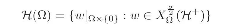
The domain of the natural fractional Laplacianis the space H(Ω)defined by
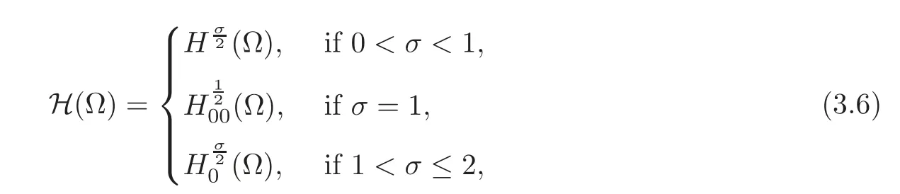
whereandare usual fractional Sobolev spaces(see[40]),and
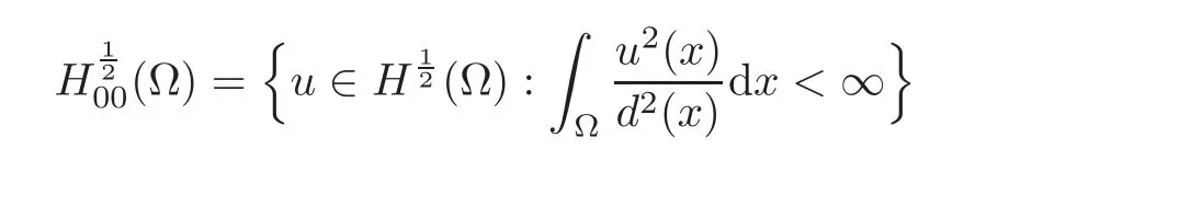
with d(x)=dist(x,∂Ω).It turns out that
(see[10]for a detailed account on this question).Then we provide the following definition.
Definition 3.1LetΩ be an open bounded set of RNand f ∈ L1(Ω).We say that w ∈is a weak solution to(3.2)if TrΩ(B(w))=:B(w(x,0))∈L1(Ω)and

for all the test functionssuch that TrRN(ϕ)≡ 0 in RNΩ.
If w is a solution to the “extended problem” (3.2),then the trace function v=TrΩ(w)will be called a weak solution to(3.1).
Remark 3.1It is clear that if B(t)=ct for all t≥0 for some c≥0,then(3.2)becomes linear and the function v=TrΩ(w)belongs to the space H(Ω).
Concerning existence of solutions,their smoothness and L1contraction properties,we excerpt some known results from[10,26–27]which can be extended for our more general nonlinearity B.For the regularity,the reader may consult[16,18,50–52].
Theorem 3.1For any f ∈ L∞(Ω),there exists a unique weak solutionto(3.2),such that TrΩ(B(w))∈ L∞(Ω).Moreover,we have the following:
(i)Regularity.We have w ∈ Cα(CΩ)for everyα < σ ifσ ≤1(resp.w ∈C1,α(CΩ)for every α<σ−1 ifσ>1).Arguing as in[17],the higher regularity of w depends easily on the higher regularity of f and B.
(ii)L1contraction.If w,are the solutions to(3.2)corresponding to datathe following L1contraction property holds:

In particular,we have that w≥ 0 inwhenever f≥ 0 onΩ.Furthermore,if we put u:=B(w(·,0)),then for all p ∈ [1,∞],we have

(iii)For f ∈ L1(Ω),the weak solution is obtained as the limit of the solutions of approximate problems with fn∈ L1(Ω)∩L∞(Ω),fn→ f in L1.Then the sequence{B(wn(x,0))}nalso converges in L1to some B(w(x,0)),and?B(w(x,0))?1≤?f?1,and hence vnis uniformly bounded in Lpfor all small p.Property(ii)holds for such limit solutions.
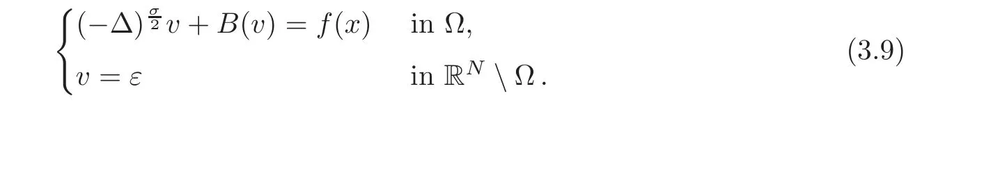
Remark 3.2(On Some Nonhomogeneous Boundary Value Problems)Letε>0.For our arguments it is essential to consider problems with nonhomogeneous boundary values of the type
In order to ensure the existence of a solution to this problem,we associate it with the following nonhomogeneous extension problem:
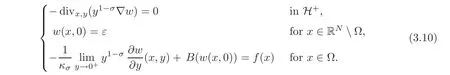
If f∈L1(Ω),we say thatis a weak solution to(3.10)ifand w satisfies(3.7).In such case,we say that v=TrΩw is a weak solution to(3.9).In particular,if B(t)=ct for all t≥0 and some c>0,and v is the solution to the following linear problem with homogeneous boundary data:
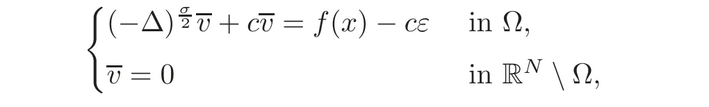
thenthe unique solution to the linear,nonhomogeneous problem(3.9).
Using the variational formulation to(3.10),it is easy to prove that ifε>0,vεis the unique weak solution to(3.9)and wεis its extension solving(3.10),then
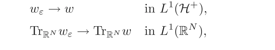
where v and w solve(3.1)and(3.2),respectively.
We warn the reader that the solutions of all the Dirichlet problems throughout this paper are identified with their extension on the whole RN,whose values out ofΩclearly depend on the boundary conditions considered.
4 Concentration Comparison for the Extended Problem
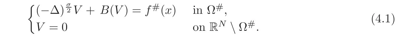
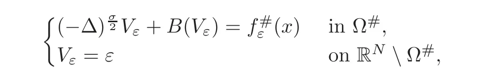
Let us address the comparison issue.From now on,we always assume that the right-hand side f is nonnegative.Our goal here is to compare the solution v to(3.1)with the solution V to the problem
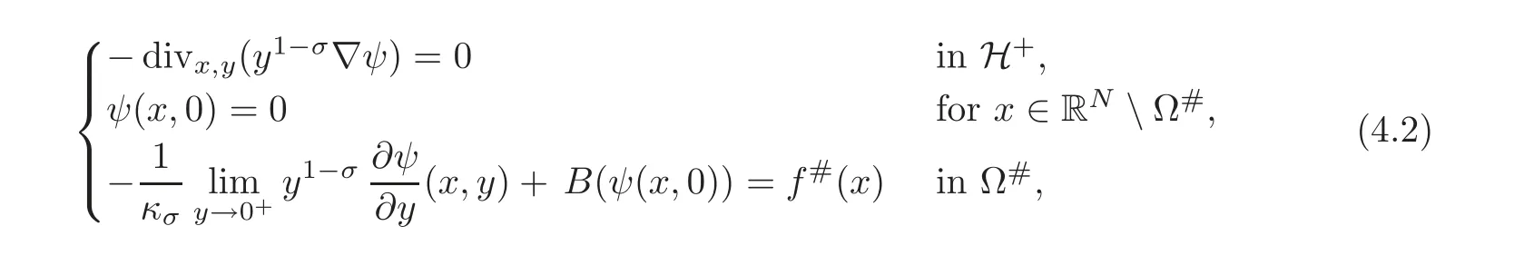
A reasonable way to do that is to compare the solution w to(3.2)with the solutionψto the problem
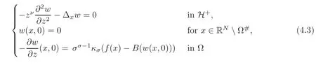
and
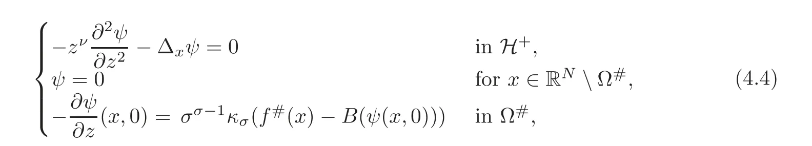
respectively,whereThen,the problem reduces to prove the concentration comparison between the solutions w(x,z)andψ(x,z)to(4.3)and(4.4),respectively.We now introduce the function
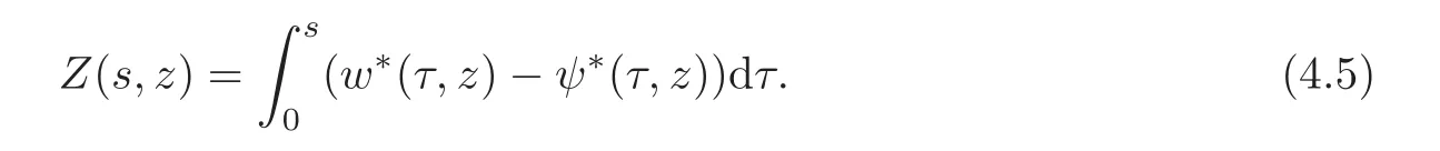
Using standard symmetrization tools(see[25]),we get the differential inequality

for a.e.(s,z)∈(0,+∞)×(0,+∞),where.Obviously,we have

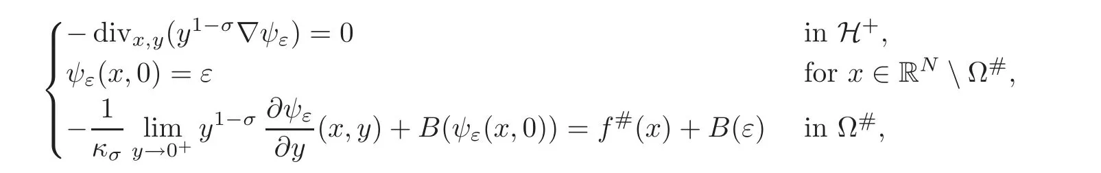
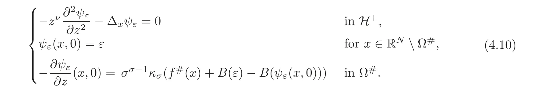
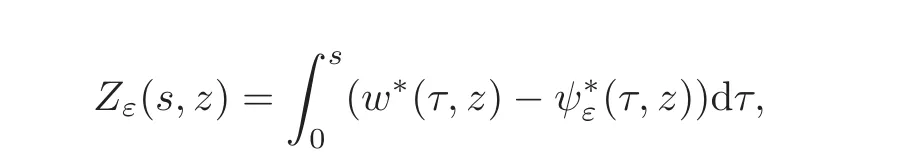
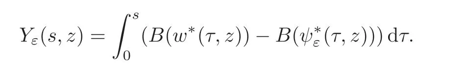
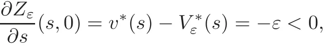
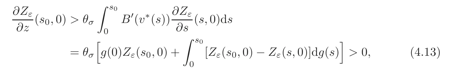
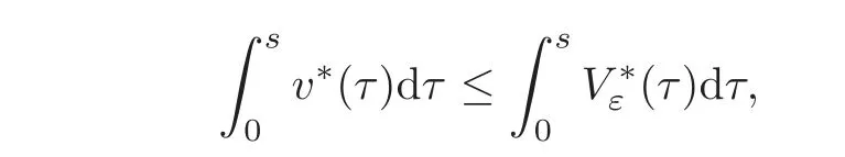
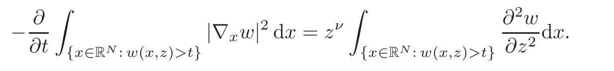
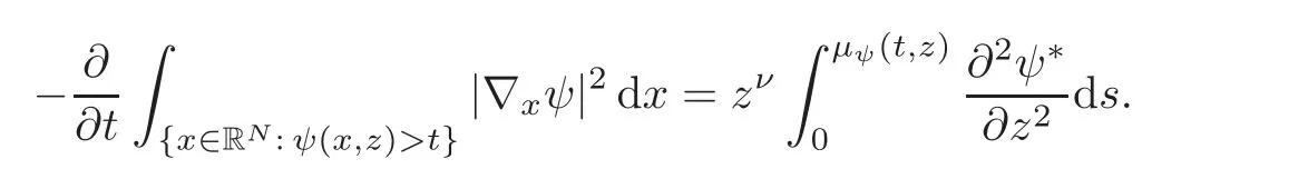
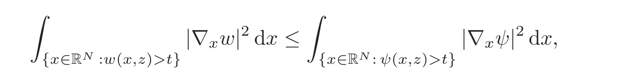
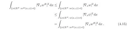
A crucial point in our arguments below is played by the derivative of Z with respect to z.Due to the boundary conditions contained in(4.3)–(4.4),we have for 0 whereOn the other hand,for s ≥ |Ω|,we haveThis is the novelty in the argument with respect to the spectral case treated before,where the boundary condition made the real difference as follows:The boundary conditions are imposed on y=0 and are of two types.Contradiction must be obtained after taking into account the two possibilities. We are going to obtain a comparison result for some linear and nonlinear B.Actually the nonlinearities considered here allow to get a result which is weaker than the one for the linear problem,i.e.,when B(t)=ct for some c≥0,which is the only case that we are going to need in addressing the Faber-Krahn inequalities.We also point out that,in order to reach our goal,we use a lifting-type argument of the symmetrized problem(4.1). Theorem 4.1Let v be the nonnegative solution to(3.1)posed in a bounded domain with zero Dirichlet boundary condition,nonnegative data f ∈ L1(Ω)and B being smooth,concave,strictly increasing on R+and such that B(0)=0.If V is the solution of the corresponding symmetrized problem(4.1),we have The same is true ifΩ=RN. ProofIn this case,we pose the problem first in a bounded domainΩof RNwith smooth boundary.We also assume that f is smooth,bounded and compactly supported inΩ,since the comparison result for general data can be obtained later by approximation,using the L1dependence on the mapLet us choose ε>0,fε=f+B(ε),and let us consider the solution Vεto the following problem: whereBy virtue of Remark 3.2,we have Vε= ψε(x,0)for all x ∈ RN,where ψεis the solution to the following problem: which can be reduced to the following problem: Setting we prove that To this aim,we first observe that Zεsatisfies(4.6).In particular,a big role is played by the property of the solution ψε:The level sets{x ∈ RN:ψε(x,z)>t}are bounded,because they are balls centered at the origin.Now we set From(4.8),we obtain By the strong maximum principle applied to(4.6),which is satisfied by Zε,a positive maximum of Zεcannot be achieved at an interior point,hence it must be achieved either as s→∞or at a boundary point(s0,0)for some s0>0.The first option cannot hold,since w∗(s,z)→ 0 whileψε(s,z)→ εas s→ ∞.As for the second,we see that for s≥ |Ω|,we have the function Zε(s,0)is strictly decreasing in[|Ω|,∞),then it must happen that s0∈ (0,|Ω|].Arguing as in[64],using(4.12),we can write where g(s):=B?(v∗(s)),which is impossible due to Hopf’s boundary maximum principle. Finally,by(4.11),we have,for s≥0, and thus asε→0, Then the result follows.The caseΩ=RNwas solved in[64,Theorem 3.2],to which the interested reader can refer. Remark 4.1If we consider the linear case,i.e.,when B(t)=ct,for some c≥0,the proof of Theorem 4.1 can be simplified,because Zε=cYε.Moreover,ψε= ψ +ε,whereψ solves(4.4),and Vε=V+ε. Remark 4.2If B is nonlinear and satisfies the assumptions of Theorem 4.1,the mass concentration comparison(4.9)is not enough to obtain the same result when it is passing to the evolution problem via Crandall-Liggett theorem. A valuable property we are going to prove now is that the equality in(4.9)implies that the domainΩof the initial problem(3.1)is actually a ball modulo translation.This kind of property is known to be essential for studying the equality case in the Faber–Krahn inequality,i.e.,to prove that the ball is the unique minimizer of the principal eigenvalue of the classical Laplacian over all the sets of fixed Lebesgue measure(see[37]). Proposition 4.1(Case of Equality)Assume that we have an equality sign in(4.9),in the sense that for all s∈ [0,|Ω|].Then Ω is a ball,i.e.,Ω = Ω#(up to a translation of the origin). ProofUsing the same notation as in Theorem 4.1,by the given assumption,we have Y(s,0)=0 for all s ∈ [0,|Ω|],and since the extensions are null,this equality holds for every s≥0.Then by Hopf’s maximum principle and(4.8),we find Y ≡ 0,and thus We divide the rest into the following steps. (i)Here we argue as in[54]or in[43].Recall that the function w(·,z)is smooth on RNfor any z>0.Then let us fix z>0,multiply both sides of the equation(4.3)by the test function and integrate over RN.An integration by parts yields the identity Then,if we let h→0,we find Thus using the second order derivation formula(see Section 7),we get Concerning the solutionψto(4.4),since it is spherically decreasing w.r.t.x,the following equality occurs: Using the fact that w∗(s,z)= ψ∗(s,z)(which implies μw(·,z)= μψ(·,z)),we have Integrating between t and∞,we find and then by the Pólya-Szegö inequality and(4.14), We conclude that for every t>0, which is the equality case in the Pólya-Szegö inequality. (ii)Now we notice that w(·,z)is analytic on the upper half space as a consequence of its representation formula.Indeed,the Poisson kernel for the extension operator Lσis given by (see,e.g.,[18]),which is an analytic function on the upper half-space z>0.This means that for every h(x)∈L1(RN),the solution w(x,z)of the elliptic equation with data w(x,0)=h(x)is analytic,since it is the convolution of h with P(with respect to the x variable).In fact,once we know that w∈C∞in a certain subdomain,it is analytic by classical results on solutions of elliptic equations with analytic coefficients(see for instance[33,35,46]). (iii)Moreover,each level set{x ∈ RN:w(x,z)>t}is bounded,because w(·,z)decays to zero as|x|→ ∞.We may now use the equality case in the Pólya-Szegö inequality(see[14,30])to obtain that{x∈RN:w(x,z)>t}={x∈RN:w#(x,z)>t}modulo a translation.Then all the level sets{x∈RN:w(x,z)>t}are balls.The results also imply that for every fixed z>0 the function w(·,z)is radially symmetric up to translation. (iv)Finally,we take the limit z→0,and we conclude that u(x)is also radially symmetric(as a function defined in RN).This means that the domainΩ,which is the positivity set of u in RN,must be a ball,i.e.,Ω=Ω#,up to a translation of the origin. The following result can be shown as in the proof of[64,Theorem 3.3] Theorem 4.2(Comparison of Concentrations for Radial Problems)Let v1,v2be two nonnegative solutions to(3.1)posed in a ball BR(0),with R∈(0,+∞]with zero Dirichlet boundary conditions if R<+∞,nonnegative radially symmetric decreasing data f1,f2∈L1(BR(0))and B(t)=ct for some c>0 and all t≥0.Then v1and v2are rearranged,and The theory of the existence of weak solutions for the initial value problem with A(u)=cum,and all c,m>0,was addressed by the first author and collaborators in[10],and the main properties were obtained.In particular,if we take initial data in L1∩H−s,then an H−s-contraction semigroup is generated,and the Crandall-Liggett discretization theorem applies.The construction and properties of the solutions of the evolution problem is thus reduced to an iterated application of the results obtained for the elliptic counterpart in the previous section.This was carefully explained in[64]and is reviewed in Subsection 7.3.Thus,using Theorem 7.2 in Subsection 7.3,we obtain the existence of a unique mild solution to the linear Cauchy-Dirichlet problem on the bounded domainΩas follows: obtained as a limit of discrete approximate solutions by the ITD scheme. Concerning the application of symmetrization techniques to this type of parabolic problems,we can employ Theorems 4.1–4.2 and the arguments in the proof of[64,Theorem 5.3]in order to find the following result. Theorem 5.1(Concentration Comparison)Let u be the nonnegative mild solution to(5.2),0< σ<2,posed inΩ,with initial data u0∈L1(Ω),and the right-hand sideAssume thatis rearrangedis rearranged w.r.t.any t>0,such that and for a.e.t>0.Let v be the solution of the evolution problem Then,for all t>0,we have In particular,we have?u(·,t)?p≤ ?v(·,t)?pfor every t>0 and every p ∈ [1,∞]. Remark 5.1The parabolic result only covers the linear equation,which is much below our original expectations,since the elliptic result covers indeed nonlinear equations.We do not know if the lack of nonlinear results is due to a failure of the expected form of the theorem,as copied from(5.1),or is only due to a lack of technique.We remind the reader that in the case of the problem in the whole space,we are able to prove the nonlinear symmetrization result when A is concave,and to show that the corresponding statement for A convex is false,so that the question is posed about which kind of statement could be true.Such question is broader in the present case. Here we prove the validity of the Faber-Krahn inequality for the fractional Laplacian operator L2defined on bounded domains of RNwith zero Dirichlet boundary conditions.This operator appears often in theory and applications,and is known under the name of restricted fractional Laplacian,though we can call it the natural fractional Laplacian.Unlike the spectral Laplacian L1,the spectral sequence{λk(L2;Ω)}kis not directly related to the sequence of the standard Laplacian.However,it is known that the spectrum is discrete and given by a strictly increasing sequence(see,e.g.,[10]).Our theorem is then stated as follows. Theorem 6.1We have with equality if and only ifΩ=Ω#,up to translation. The proof we present here is completely elementary and uses neither the variational characterization(6.6)nor the nonlocal Pólya-Szegö inequality as in[13],but only the concentration comparison provided by Theorem 5.1 and the asymptotic definition ofwhich can be derived by the decay rate of the parabolic problem Proof of Theorem 6.1Suppose thatare the(L2normalized)eigenfunctions of L2and let us consider the function solving the problem By Theorem 5.1 we find,for all t>0, where v solves the problem Since and the expression for v can be given in terms of superposition,namely, we have This together with(6.4)implies(6.1). The case of equalityAnalyzing the last list of inequalities that starts bywe conclude that in the case wherewe necessarily have so that we conclude that the coefficients of the Fourier expansion of v0=v(·,0)in terms of eigenfunctions are all zero but the first,in view of the known fact that the first eigenvalueis simple.This means thatwith a constant c>0.By normalization,we get But this is enough to apply the important Proposition 4.1 and obtainΩ=Ω#,and the result ends as before. A direct proof of the FKI for our operator and similar can be based on the variational interpretation of the first eigenvalue,since it can be written as the minimizer of the Rayleigh quotient,where the local L2gradient energy norm is replaced by the Gagliardo seminorm(see Section 7 for some details). As in the proof of Theorem 6.1,suppose thatare the(L2normalized)eigenfunctions of L2.As already mentioned in the introduction,the proof of Theorem 6.1 is a direct consequence of the variational characterization ofIndeed,we know by[48]that Then we could use the nonlocal(hence fractional)version of the Pólya-Szegö inequality(see for instance[45])to see that replacing u with u#makes the Gagliardo seminorm in(6.6)decrease,therefore(6.1)holds.Furthermore,if equality occurs in(6.1),the minimality ofimplies thatis an eigenfunction.But since the eigenvalueis also simple,by normalization,we have which the same result in[45]shows to be possible only when Ω = Ω#andup to translation. M ore general version of the FK IActually,Brasco et al.[13]was able to establish a more general version of the FKI,which applies to a nonlinear variant of the fractional Laplacian,namely the fractional p-Laplacian.The main argument of the general variational proof is the use of a nonlocal Pólya-Szegö inequality,proved in[32],to estimate the first nonlinear eigenvalue. Probabilistic approachThe Faber-Krahn inequality for the fractional Laplacian with Dirichlet data on a bounded domain of RNis stated with a hint of the proof based on probabilistic arguments as the last result(see[4,Theorem 5]).This means that the eigenvalues are also characterized in terms of the evolution,in their case of the stochastic process of Levy type.Another proof with probabilistic flavor can be found in[9]. We gather here some basic information on symmetrization that can be useful to read this paper.We follow standard notations used in this literature,and we recall that we presented a more detailed account in[64].A measurable real function f defined on RNis called radially symmetric(radial,for short)if there is a functionsuch thatfor all x∈RN.We often writefor such functions by abuse of notation.We say that f is rearranged if it is radial,nonnegative andis a right-continuous,non-increasing function of r>0.A similar definition can be applied for real functions defined on a ball IfΩ is an open set of RNand f is a real measurable function on Ω,we denote by|·|the N-dimensional Lebesgue measure.We define the distribution functionμfof f as and the decreasing rearrangement of f as We may also think of extending f∗as the zero function in[|Ω|,∞)ifΩ is bounded.From this definition,it turns out thatμf∗= μf(i.e.,f and f∗are equi-distributed)and f∗is exactly the generalized inverse ofμf.Furthermore,ifωNis the measure of the unit ball in RNand Ω#is the ball of RNcentered at the origin having the same Lebesgue measure asΩ,we define the function which is called spherical decreasing rearrangement of f.From this definition,it follows that f is rearranged if and only if f=f#. Rearranged functions have a number of interesting properties.Here,we just recall the conservation of the Lpnorms(coming from the definition of rearrangements and the classical Cavalieri principle):For all p∈ [1,∞], as well as the classical Hardy-Littlewood inequality(see[34]) (1)We often deal with two-variable functions of the type defined on the cylinder CΩ:=Ω×(0,+∞),and measurable with respect to x.HereΩcan be a bounded domain or RN.For such functions,it is convenient to define the so-called Steiner symmetrization of CΩwith respect to the variable x,namely the setFurthermore,we denote by μf(k,y)and f∗(s,y)the distribution function and the decreasing rearrangements of(7.2),respectively,with respect to x for y fixed,and we also define the function which is called the Steiner symmetrization of f,with respect to the line x=0.Clearly,f#is a spherically symmetric and decreasing function with respect to x,for any fixed y. (2)There are some interesting differentiation formulas which turn out to be very useful in our approach.Typically,they are used when one wants to get sharp estimates satisfied by the rearrangement u∗of a solution u to a certain equation,and it becomes crucial to differentiate with respect to the extra variable y(introduced in the extension process that is used in fractional operators)in the form We recall here two formulas that have been already used in[25,64]. Proposition 7.1Suppose that f ∈ H1(0,T;L2(Ω))for some T>0 and f is nonnegative.Then If|{f(x,t)=f∗(s,t)}|=0 for a.e.(s,t)∈ (0,|Ω|)×(0,T),the following differentiation formula holds: The second-order differentiation formula is as follows. Proposition 7.2Let f be nonnegative and f ∈ W2,∞(CΩ).Then for almost every y ∈(0,+∞)the following differentiation formula holds: (3)Mass concentration.We provide estimates of the solutions of our elliptic and parabolic problems in terms of their integrals.For that purpose,the following definition,taken from[58],is remarkably useful. Definition 7.1Letbe two radially symmetric functions on RN.We say that f is less concentrated than g,and we writeif for allwe get The partial order relationshipis called comparison of mass concentrations.Of course,this definition can be suitably adapted if f,g are radially symmetric and locally integrable functions on a ball BR.Besides,if f and g are locally integrable on a general open setΩ,we say that f is less concentrated than g,and we write againsimply ifbut this extended definition has no use if g is not rearranged. The comparison of mass concentrations enjoys a nice equivalent formulation if f and g are rearranged,whose proof we refer to[21,34,59]. Lemma 7.1Let f,g ∈ L1(Ω)be two rearranged functions on a ballΩ =BR(0).Thenif and only if for every convex nondecreasing functionwithΦ(0)=0 we have This result still holds if R=∞andwith g→0 as|x|→∞. From this lemma it easily follows that if f≺g and f,g are rearranged,then In the analyticity argument of Proposition 4.1,we want to apply the results of[35].Let us put where subindexes indicate partial derivatives.Then,for each j=1,···,N andfor j?=k.Thus for allThen the equation is elliptic in.Since a solution w to such equation is C∞inand the functionis analytic inwe can apply the main theorem in[35]and conclude that w(x,z)is analytic in Let X be a Banach space and A:D(A)⊂X→X be a nonlinear operator defined on a suitable subset of X.Let us consider the problem where u0∈X and f∈L1(I;X)for some interval I of the real axis.For a wide class of operators,in particular the ones considered in this paper,a very efficient way to approach such problem is to use an implicit time discretization scheme that we describe next.Suppose to be specific that I=[0,T](but this can be replaced by any interval[a,b]and the procedure is similar).The method consists in taking first a partition of the interval,say,tk=kh for k=0,1,···,n and,and then solving the system of difference relations for k=0,1,···,n,where we pose uh,0=u0.The data setis supposed to be a suitable discretization of the source term f,corresponding to the time discretization we choose.This process is called implicit time discretization scheme(ITD for short)of the equation u?(t)+A(u)=f.It can be rephrased in the form where the operator Jλ=(I+ λA)−1,λ >0 is called the resolvent operator,with I being the identity operator.Therefore,the application of the method needs the operator A to have a well-defined family of resolvents with good properties.When the ITD is solved,we construct a discrete approximate solution{uh,k}k.By piecing together the values uh,k,we take a piecewise constant function,uh(t),typically defined through (or some other interpolation rule,like linear interpolation).Then the main question consists in verifying if such function uhconverges somehow as h→0 to a solution u(which we hope to be a classical,strong,weak,or other type of solution)to(7.6).To this regard,we first choose a suitable discretizationin time of the source term f,such that the piecewise constant interpolation of this sequence produces a function f(h)(t)(defined by means of(7.8))verifies the property By means of these discrete approximate solutions,we introduce the following notion of mild solution. Definition 7.2We say that u∈C((0,T);X)is a mild solution to(7.6)if it is obtained as uniform limit of the approximate solutions uh,as h→0.The initial data are taken in the sense that u(t)is continuous in t=0 and u(t)→u0as t→0.Besides,we say that u∈C((0,∞);X)is a mild solution to(7.6)in[0,∞)if u is a mild solution to the same problem in any compact subinterval I⊂ [0,∞). In order to state a positive existence result,we need to restrict the class of operators according to the following definitions. Definition 7.3Let A:D(A)⊂X→X be a nonlinear,possibly unbounded operator.Let Rλ(A)be the range of I+λA,a subset of X. (i)The operator A is said accretive if for allλ >0 the map I+λA is one-to-one onto Rλ(A)⊂ X,and the resolvent operator Jλ:Rλ(A)→ X is a(non-strict)contraction in the X-norm(i.e.,a Lipschitz map with Lipschitz norm 1). (ii)We say that A satisfies the rank condition iffor allλ>0.In particular,the rank condition is satisfied if Rλ(A)=X for allλ >0.In this case,if A is accretive,we say that A is m-accretive. We are now ready to state the desired semigroup generation result,that generalizes the classical result of Hille-Yosida(valid in Hilbert spaces and for linear A)and the variant by Lumer and Phillips(valid in Banach spaces,still for linear A),and provides the existence and uniqueness of mild solutions to problems of the type(7.6)in the case f≡0. Theorem 7.1(Crandall-Liggett)Suppose that A is an accretive operator satisfying the rank condition.Then for all datathe limit exists uniformly with respect to t,on compact subset of[0,∞),and u(t)=St(A)u0∈ C([0,∞):X).Moreover,the family of operators{St(A)}t>0is a strongly continuous semigroup of contractions on Using a popular notation in the linear framework,we could write,and because of this analogy formula,(7.9)is called the Crandall-Liggett exponential formula for the nonlinear semigroup generated by−A.The problem with this very general and useful result is that the X-valued function u(t)=St(A)u0solves the equation only in a mild sense,which is not necessarily a strong solution or a weak solution.Though it is known that strong solutions are automatically mild,the correspondence between mild and weak solutions is not always clear.For the FPME,this issue was discussed in detail in[26–27]. In addition,the Crandall-Liggett theorem result can be extended when we consider nontrivial source term f,according to the following result. Theorem 7.2Suppose that A is m-accretive,f∈ L1(0,∞;X)andThen the abstract problem(7.6)has a unique mild solution u,obtained as the limit of the discrete approximate solution uhby ITD scheme described above,as h→0, and the limit is uniform in compact subsets of[0,∞).Moreover,u ∈ C([0,∞);X)and for any couple of solutions u1,u2corresponding to source terms f1,f2,we have for all 0≤s There is a wide literature on these topics,starting with the seminal paper by Crandall and Liggett[24](see also[23]and the general reference[5]).These notes are based on[60,Chapter 10](see the references therein).The last formula we mentioned introduces the correct concept of uniqueness for the constructed class of solutions.Characterizing the uniqueness of different concepts of solution is a difficult topic already discussed(with positive results)by Bénilan[6]. (1)We have only proved results on parabolic comparison based on symmetrization for the linear case.The elliptic results can be applied to nonlinear equations but still have severe restrictions.It is interesting to know how much is true for nonlinear functions B and A in the respective equations.This question was partially addressed and solved for the spectral fractional Laplacian in[64],and the limitations to the generality of the results were also shown to be necessary,the symmetrization result was false for the concave B or the convex A of power type. More generally,we would like to know if there is an approach that ensures comparison results of some symmetrization type valid for quite general nonlinearities,as it happens in the non-fradtional case(see[59]). (2)The variable coefficient case.As a future direction,we are interested in the following problem: where Here the matrix A(x)is supposed to be W1,∞(RN)and uniformly elliptic with lower constant Λ>0. It is a well-known fact that the spectral powers of div(A(x)∇),i.e.,(div(A(x)∇))sfor s∈(0,1)in a bounded domainΩcan be described as the Dirichlet-to-Neumann operator of a suitable extension in a cylinder C=Ω×R+(see for instance[19]for a detailed account).The previous problem(8.1)is a variant of this extension but in the whole RN.The Dirichletto-Neumann operator in this case is not explicitly identified.However,we believe that it is a natural possible extension of the problem we considered in this paper.The idea here is to develop the techniques produced in the present paper to handle variable coefficients,having in mind an isoperimetric inequality.Indeed,an FKI is proven in terms of the first eigenvalue by means of The aim here is to prove such a result for the following problem:Let Lsbe the Dirichlet-to-Neumann operator associated to(8.1)defined onΩ.It is obvious that Lshas discrete spectrumIt is not clear how to use a variational approach to deal with this operator,since it does not seem obvious that this operator is associated to a norm in RNsatisfying a Pólya-Szegö inequality.However,the parabolic approach developed in the present paper seems promising. [1]Applebaum,D.,Lévy processes and stochastic calculus,Cambridge Studies in Advanced Mathematics,2nd edition,116,Cambridge University Press,Cambridge,2009. [2]Bandle,C.,Isoperimetric inequalities and applications,Monographs and Studies in Mathematics,7,Pitman(Advanced Publishing Program),Boston,London,1980. [3]Bandle,C.,On symmetrizations in parabolic equations,J.Analyse Math.,30,1976,98–112. [4]Banuelos,R.,Latala,R.and Méndez-Hernández,P.J.,A Brascamp-Lieb-Luttinger-type inequality and applications to symmetric stable processes,Proc.Amer.Math.Society,129(10),2001,2997–3008. [5]Barbu,V.,Nonlinear Semigroups and Differential Equations in Banach Spaces,Noordhoff,Leyden,1975. [6]Bénilan,Ph.,Equations d’évolution dans un espace de Banach quelconque et applications(in French),Ph.D.Thesis,Univ.Orsay,1972. [7]Bertoin,J.,Lévy processes,Cambridge Tracts in Mathematics,121,Cambridge University Press,Cambridge,1996. [8]Bénilan,P.,Brezis,H.and Crandall,M.G.,A semilinear equation in L1(RN),Ann.Scuola Norm.Sup.Pisa Cl.Sci.,2(4),1975,523–555. [9]Betsakos,D.,Symmetrization,symmetric stable processes,and Riesz capacities(electronic),Trans.Amer.Math.Soc.,356,2004,735–755. [10]Bonforte,M.,Sire,Y.and Vázquez,J.L.,Existence,uniqueness and asymptotic behaviour for fractional porous medium equations on bounded domains,Discrete Contin.Dyn.Syst.A,35(12),2015,5725–5767. [11]Bonforte,M.and Vázquez,J.L.,Quantitative local and global a priori estimates for fractional nonlinear diffusion equations,Advances in Math.,250,2014,242–284. [12]Bonforte,M.and Vázquez,J.L.,A priori estimates for fractional nonlinear degenerate diffusion equations on bounded domains,Arch.Ration.Mech.Anal.,218(1),2015,317–362. [13]Brasco,L.,Lindgren,E.and Parini,E.,The fractional Cheeger problem,Interfaces Free Bound.,16(3),419–458. [14]Brothers,J.and Ziemer,W.,Minimal rearrangements of Sobolev functions,J.Reine Angew.Math.,384,1988,153–179. [15]Bucur,D.and Freitas,P.,A new proof of the Faber-Krahn inequality and the symmetry of optimal domains for higher eigenvalues,2012,preprint. [16]Cabré,X.and Sire,Y.,Nonlinear equations for fractional Laplacians,I:Regularity,maximum principles,and Hamiltonian estimates,Ann.Inst.H.Poincaré Anal.Non Linéaire,31(1),2014,23–53. [17]Cabré,X.and Tan,J.G.,Positive solutions of nonlinear problems involving the square root of the Laplacian,Adv.Math.,224(5),2010,2052–2093, [18]Caffarelli,L.and Silvestre,L.,An extension problem related to the fractional Laplacian,Comm.Part.Diff.Eq.,32(7–9),2007,1245–1260. [19]Caffarelli,L.and Stinga,P.,Fractional elliptic equations,Caccioppoli estimates and regularity,Ann.Inst.H.Poincaré Anal.Non Linéaire,33(3),2016,767–807. [20]Chavel,I.,Eigenvalues in Riemannian Geometry,Series in Pure and Applied Mathematics,115,Academic Press,Orlando,1984. [21]Chong,K.M.,Some extensions of a theorem of Hardy,Littlewood and Pólya and their applications,Canad.J.Math.,26,1974,1321–1340. [22]Brändle,C.,Colorado,E.and de Pablo,A.,A concave-convex elliptic problem involving the fractional laplacian,Proceedings of the Royal Society of Edinburgh,143A,2013,39–71. [23]Crandall,M.G.,Nonlinear semigroups and evolution governed by accretive operators,Proceedings of Symposium in Pure Math.,Part I,F.Browder(ed.),A.M.S.,Providence,RI,1986,305–338. [24]Crandall,M.G.and Liggett,T.M.,Generation of semi-groups of nonlinear transformations on general Banach spaces,Amer.J.Math.,93,1971,265–298. [25]Di Blasio,G.and Volzone,B.,Comparison and regularity results for the fractional Laplacian via symmetrization methods,J.Differential Equations,253(9),2012,2593–2615. [26]De Pablo,A.,Quirós,F.,Rodríguez,A.and Vázquez,J.L.,A fractional porous medium equation,Adv.Math.,226(2),2011,1378–1409. [27]De Pablo,A.,Quirós,F.,Rodríguez,A.and Vázquez,J.L.,A general fractional porous medium equation,Comm.Pure Appl.Math.,65(9),2012,1242–1284. [28]De Pablo,A.,Quirós,F.,Rodríguez,A.and Vázquez,J.L.,Classical solutions for a logarithmic fractional diffusion equation,preprint. [29]De Pablo,A.,Quirós,F.,Rodríguez,A.and Vázquez,J.L.,Classical solutions and higher regularity for nonlinear fractional diffusion equations,JEMS,to appear. [30]Ferone,A.and Volpicelli,R.,Minimal rearrangements of Sobolev functions:A new proof,Ann.Inst.H.Poincaré Anal.Non Linéaire,20(2),2003,333–339. [31]Faber,C.,Beweiss,dass unter allen homogenen Membrane von gleicher Fläche und gleicher Spannung die kreisförmige die tiefsten Grundton gibt,Sitzungsber.Bayer.Akad.Wiss.,Math.Phys.Munich.,1923,169–172. [32]Frank,R.L.and Seiringer,R.,Non-linear ground state representations and sharp Hardy inequalities,J.Funct.Anal.,255,2008,3407–3430. [33]Friedman,A.,On the regularity of the solutions of nonlinear elliptic and parabolic systems of partial differential equations,J.Math.Mech.,7,1958,43–59. [34]Hardy,G.H.,Littlewood,J.E.and Pólya,G.,Some simple inequalities satisfied by convex functions,Messenger Math.,58,1929,145–152,Inequalities,2nd edition,Cambridge University Press,Cambridge,1952. [35]Hashimoto,Y.,A remark on the analyticity of the solutions for non-linear elliptic partial differential equations,Tokyo J.Math.,29(2),2006,271–281. [36]Kawohl,B.,Rearrangements and convexity of level sets in PDE,Lecture Notes in Mathematics,1150,Springer-Verlag,Berlin,1985. [37]Kesavan,S.,Symmetrization and applications,Series in Analysis,Vol.3,World Scientific Publishing,Hackensack,NJ,2006. [38]Krahn,E.,Uber eine von Rayleigh formulierte Minmaleigenschaft des Kreises,Math.Ann.,94,1925,97–100. [39]Landkof,N.S.,Foundations of modern potential theory,Die Grundlehren der Mathematischen Wissenschaften,Band 180,Springer-Verlag,New York,Heidelberg,1972. [40]Lions,J.-L.and Magenes,E.,Non-homogeneous boundary value problems and applications.Vol.I,GMW 181,Springer-Verlag,New York,Heidelberg,1972. [41]Luttinger,J.M.,Generalized isoperimetric inequalities,Proc.Nat.Acad.Sci.U.S.A.,70,1973,1005–1006. [42]Maz’ja,V.G.,Weak solutions of the Dirichlet and Neumann problems(in Russian),Trudy Moskov.Mat.Ob˘suc.,20,1969,137–172. [43]Mossino,J.and Rakotoson,J.-M.,Isoperimetric inequalities in parabolic equations,Ann.Scuola Norm.Sup.Pisa Cl.Sci.,13(4),1986,51–73. [44]Musina,R.and Nazarov,A.I.,On fractional Laplacians,Comm.Part.Diff.Eqs.,39(9),2014,1780–1790. [45]Park,Y.J.,Fractional Pólya-Szegö inequality,J Chungcheong Math.Soc.,24(2),2011,267–271. [46]Petrowskii,I.,Sur l’analyticité des solutions des systèmes d’équations diff érentielles,Mat.Sbornik(N.S.),5(47),1939,3–70. [47]Pólya,G.and Szegö,C.,Isoperimetric inequalities in mathematical physics,Annals of Mathematics Studies,Vol.27,Princeton University Press,Princeton,N.J.,1951. [48]Servadei,R.and Valdinoci,E.,Variational methods for non-local operators of elliptic type,Discrete Contin.Dyn.Syst.,33(5),2013,2105–2137. [49]Servadei,R.and Valdinoci,E.,On the spectrum of two different fractional operators,Proc.Roy.Soc.Edinburgh Sect.A,144(4),2014,831–855. [50]Servadei,R.and Valdinoci,E.,Weak and viscosity solutions of the fractional Laplace equation,Publ.Mat.,58(1),2014,133–154. [51]Silvestre,L.E.,Hölder estimates for solutions of integro differential equations like the fractional Laplace,Indiana Univ.Math.J.,55(3),2006,1155–1174. [52]Silvestre,L.E.,Regularity of the obstacle problem for a fractional power of the Laplace operator,Comm.Pure Appl.Math.,60(1),2007,67–112. [53]Stein,E.M.,Singular integrals and differentiability properties of functions,Princeton Mathematical Series,No.30,Princeton University Press,Princeton,N.J.,1970. [54]Talenti,G.,Elliptic equations and rearrangements,Ann.Scuola Norm.Sup.,3(4),1976,697–718. [55]Talenti,G.,Nonlinear elliptic equations,rearrangements of functions and Orlicz spaces,Annal.Mat.Pura Appl.,4,120,1979,159–184. [56]Talenti,G.,Linear elliptic P.D.E.’s:Level sets,rearrangements and a priori estimates of solutions,Boll.Un.Mat.Ital.B,4(6),1985,917–949. [57]Valdinoci,E.,From the long jump random walk to the fractional Laplacian,Bol.Soc.Esp.Mat.Apl.,49,2009,33–44. [58]Vázquez,J.L.,Symétrisation pour ut= Δϕ(u)et applications,C.R.Acad.Sc.Paris,295,1982,71–74. [59]Vázquez,J.L.,Symmetrization and mass comparison for degenerate nonlinear parabolic and related elliptic equations,Advances in Nonlinear Studies,5,2005,87–131. [60]Vázquez,J.L.,The porous medium equation.Mathematical Theory,Oxford Mathematical Monographs.The Clarendon Press,Oxford University Press,Oxford,2007. [61]Vázquez,J.L.,Smoothing and decay estimates for nonlinear diffusion equations:Equations of porous medium type,Oxford Lecture Series in Mathematics and Its Applications,33,Oxford University Press,Oxford,2006. [62]Vázquez,J.L.,Nonlinear diffusion with fractional Laplacian operators,Nonlinear Partial Differential Equations:The Abel Symposium 2010,Holden,H.and Karlsen,K.H.(eds.),Springer-Verlag,New York,2012,271–298. [63]Vázquez,J.L.,Barenblatt solutions and asymptotic behaviour for a nonlinear fractional heat equation of porous medium type,J.Eur.Math.Soc.,16,2014,769–803. [64]Vázquez,J.L.and Volzone,B.,Symmetrization for linear and nonlinear fractional parabolic equations of porous medium type,J.Math.Pures Appl.,101,2014,553–582. [65]Vázquez,J.L.and Volzone,B.,Optimal estimates for fractional fast diffusion equations,J.Math.Pures Appl.(9),103(2),2015,535–556. [66]Weinberger,H.,Symmetrization in uniformly elliptic problems,Studies in Mathematical Analysis,Stanford University Press,California,1962,424–428.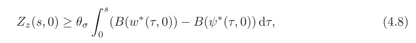

4.1 Comparison result for the elliptic problem


5 Symmetrization for the Parabolic Problem


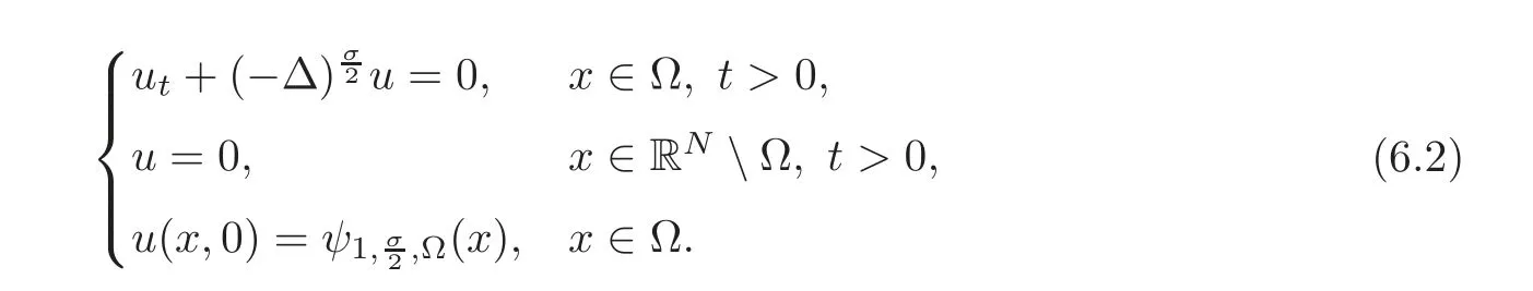
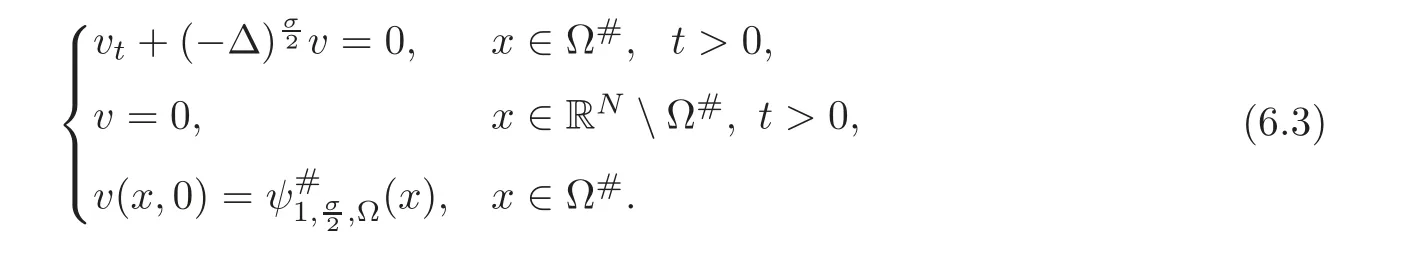
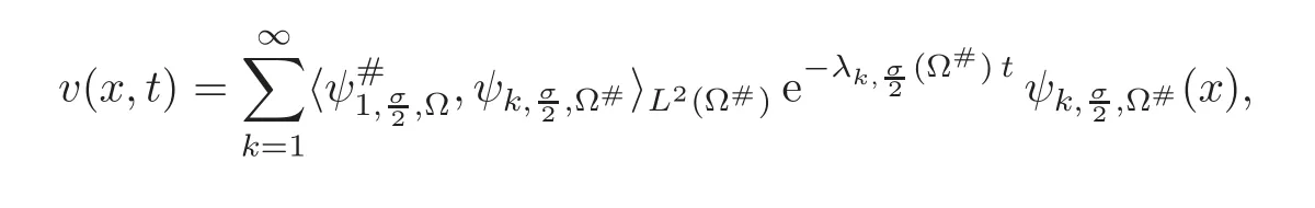
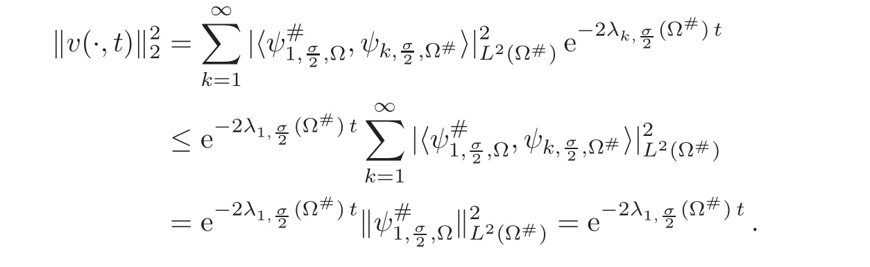
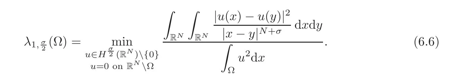
6 Application:An Original Proof of the Fractional Faber-Krahn Inequality


6.1 A variational proof
7 Appendices
7.1 On symmetrization


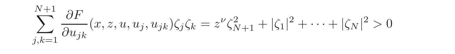
7.2 On analyticity

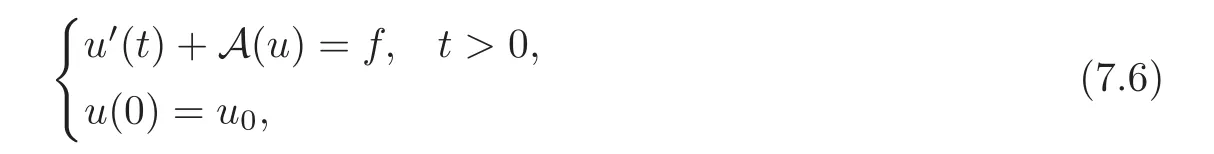
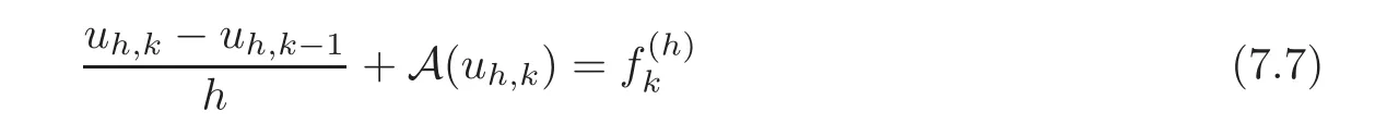
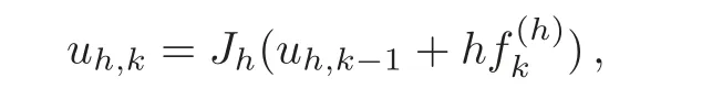
7.3 On accretive operators and the semigroup approach


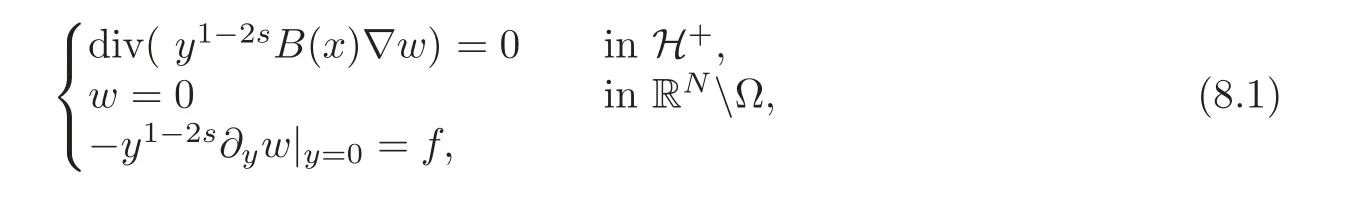
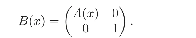
8 Comments and Extensions
杂志排行
Chinese Annals of Mathematics,Series B的其它文章
- CR Geometry in 3-D∗
- A Third Derivative Estimate for Monge-Ampere Equations with Conic Singularities
- The Mathematical Theory of Multifocal Lenses∗
- Convergence to a Single Wave in the Fisher-KPP Equation∗
- Negative Index Materials and Their Applications:Recent Mathematics Progress
- Singular Solutions to Conformal Hessian Equations