Numerical simulation of hydrodynamic performance of blade position-variable hydraulic turbine＊

Long-jing Li (李龙敬), Shen-jie Zhou (周慎杰),2

1.School of Mechanical Engineering, Shandong University, Jinan 250061, China, E-mail: kglilongjing@163.com

2.Key Laboratory of High Efficiency and Clean Mechanical Manufacture, Shandong University, Jinan 250061, China

Numerical simulation of hydrodynamic performance of blade position-variable hydraulic turbine＊

Long-jing Li (李龙敬)1, Shen-jie Zhou (周慎杰)1,2

1.School of Mechanical Engineering, Shandong University, Jinan 250061, China, E-mail: kglilongjing@163.com

2.Key Laboratory of High Efficiency and Clean Mechanical Manufacture, Shandong University, Jinan 250061, China

This paper presents a study of the movement and the hydrodynamic performance of a new tide-powered hydraulic turbine through numerical simulations. By means of the moving mesh method, the open-closed sequences of the blades and the movement of the rotors are obtained and the angular velocity and the average energy utilization coefficient under different tip speed ratios are also obtained. Moreover, the optimum tip speed ratio is identified by integrating the output power and the energy utilization coefficient of the hydraulic turbine with different tip speed ratios, providing data support for the prototype design of the hydraulic turbine.

Hydraulic turbine, blade position-variable, hydraulic performance

Introduction

In recent years, the kinetic energy stored in tide has been gradually made clear. Despite of the lower density than that of conventional energy sources, the tide energy is advantageous in many aspects, such as the eco-friendliness, the predictability, the short construction cycle and the lower cost[1], all of which are significant for the electricity generation. In the meanwhile of the gradual commercialization of the horizontal-axis hydraulic turbine[2-4], the vertical-axis hydraulic turbine[5]is also under a continuous development. The vertical-axis turbine is preferred by many designers owing to its response to the flows from different directions and is widely applied in the tide energy conversion device.

The Darrieus hydraulic turbine is one of the bestknown vertical-axis hydraulic turbines. Lam and Dai[6], Antheaume et al.[7]used the 2-D numerical simulation to successfully predict the performance of a Darrieus hydraulic turbine[8-10]. By combining the free vortex model with the finite element method (FEM) analysis to calculate the flow fields by partitions, Ponta et al.[11,12]proposed the vortex method combined with the finite element analysis, similar to the previous classic free vortex model of Strickland, in which the free vortex model and the FEM method are applied to calculations in the external larger zones and the smaller zones around the blades, respectively. Li and Çalişal[13,14]proposed the discrete vortex model based on the vortex theory and further developed the mutual interfering model of multiple hydraulic turbines based on the calculation of the single hydraulic turbine model[15,16]. In addition, the interference of two or more hydraulic turbines was also studied and related methods were verified through a series of towing tank tests[17,18]. In combination with the test results, Yang and Lawn[19,20]obtained the open-closed sequences of the hydraulic turbine blade, which has facilitated the determination of the moving state of the blades. On this basis, the flow field of the hydraulic turbine in different times was obtained by numerical simulations.

The precise prediction of the performance of the hydraulic turbine through numerical simulations provides guidance for the design of the hydraulic turbine. However, in the study of the hydraulic turbine’s hydrodynamic performance, the fixed angular velocity ratherthan the actual passive movement is often adopted for numerical simulations, with certain limits for the blade position-variable hydraulic turbine. In this paper, taking the fluid-structure interaction into consideration, the numerical simulation is performed based on the moving meshing method to investigate one single blade at different times and the instant open-closed situation of different blades. The movement of the rotor and the output power and the average energy utilization coefficient at different moments and the velocities of the incident flow are obtained, which shows the actual movement process of the hydraulic turbine.

1. Operating principle and movement analysis of hydraulic turbine

The hydraulic turbine is composed of the wheel hub, the blade and the connecting rod, as shown in Fig.1. The main innovation of the structure is in the connecting rods. In the process of movement, the connecting rods accelerate the complete opening of the blades downstream, as well as the complete closing of the blades upstream. As a result, the blades upstream can stick on the revolving drum, while the blades downstream stay upright to absorb the energy. Compared with those without the linkages, the blades open earlier, the effective incident flow area increases, therefore, the driving moment is larger.

Fig.1 Blade position-variable of hydraulic turbine

1.1Operating principle and movement analysis

As the impeller rotates, the blades upstream will stick on the revolving drum under the action of the tidal flow, while the blades downstream will stay upright under the action of the interlocking mechanism. Meanwhile, the tidal flow drives the impeller to rotate, and the engine is driven to generate electricity. The maximum driving moment can be achieved under the same tidal flow.

The force of the flow field on the hydraulic turbine can be simplified into the force and the moment on the axis. The movement of the hydraulic turbine can be expressed as:

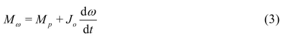
According to Eq.(3), a part of the rotor’s rotating moment is applied as the driving moment of load, while the remaining part serves as the inherent inertia moment. It should be noted thatdenotes the resultant moment of six blades, i.e.,whereas,denotes the tangential force of a single blade. The resultant moment of the blades varies with the tangential forces due to the different positions of the blades.denotes the rotational inertia, varying with the positions of the blades.

According to the analysis, the rotation of the entire rotor is a kind of variable acceleration movement varying with the positions of the blades. The movement can be determined by the open-closed locations of the blades and the angular velocity in rotation.

1.2Similarity analysis

In the process of simulation, the computation burden would be very heavy in case of modeling based on the prototype design size. Hence, the prototype size should be reduced properly based on the similarity principle with the numerical accuracy ensured. According to the similarity principle in hydrodynamics, the similarity between the model and the prototype must be guaranteed so that the model can reflect the real conditions of the prototype. Similarity criterion varies according to different objectives of study.

The main structural parameters of the hydraulic turbine proposed to be designed in this paper include the actual flow velocity of 2 m/s, the diameter of the revolving drum of 1 m and the maximum stretching chord height of the blade of 0.46 m. For the hydraulic turbine to meet the Euler and Hal similarity criteria, the size of the model is reduced 10 times for simulation. The simulated diameter of the wheel hub and themaximum stretching chord height of the blade are 100 mm and 46 mm, respectively.

2. Numerical simulation method

The blade position-variable vertical-axis hydraulic turbine is taken as the object of study, as shown in Fig.1. To study the movement of the blades and predict the hydrodynamic performance of the hydraulic turbine, the numerical simulation is performed based on the moving meshing method by virtue of workbench.

The main simulation parameters are shown in Table 1. The incompressible water is used as the working fluid and the solid part is treated as the rigid body of steel material. In the process of the fluid-structure interaction due to the system coupling, the interaction force between the fluid and the solid parts must be transmitted across the fluid-structure interaction surface. Therefore, a very small thickness is assumed in the simulation (the process can be regarded as the 2-D simulation) to create the fluid-structure interaction surface in the coupling.

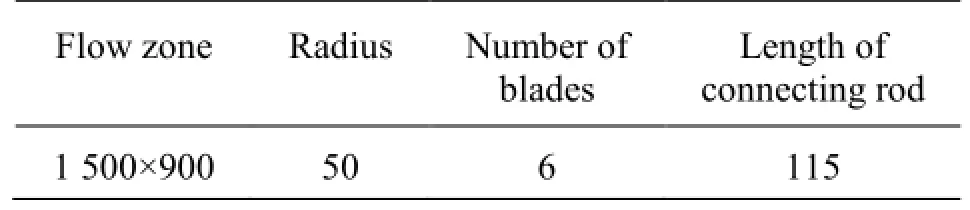
Table 1 Main sizes of the model (mm)

The coupling system provides the mechanical system with static data as well as data from co-simulation coupling participants, such as the External Data and ANSYS FLUENT systems, respectively. To do this, the Setup cell from the mechanical system is linked to the Setup cell in the coupling system. To transfer the force from the CFD pressures and the viscous forces, a co-simulation compatible coupling participant, such as the ANSYS FLUENT analysis system, is linked to the coupling system that is connected to the transient structural system. In the coupling system, the desired data are transferred from the other co-simulation coupling participant to the mechanical coupling participant.

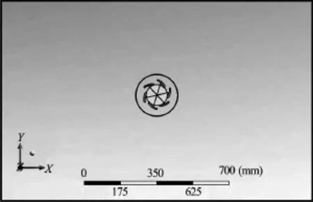
Fig.2 Flow field of hydraulic turbine

Fig.3 Locally redefined mesh of fluid zone

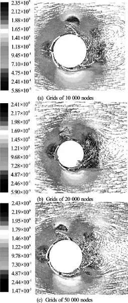
Fig.4 Different grids of nodes

In the coupling system approach, other coupling participants can also be included with data from the mechanical system. To transfer the displacement data, the transient structural system and the ANSYS FLUENT analysis system co-simulation compatible coupling participant are linked to a coupling system.In the coupling system, the desired data are transferred from the mechanical system to the ANSYS FLUENT analysis system.

As shown in Fig.2, the flow domain is meshed with tri-prism grids, the hydraulic turbine zone is locally refined as shown in Fig.3. The left side of the area is defined as the velocity inlet, the right side of the area as the pressure outlet, other areas are defined as the walls, and the outline of the hydraulic turbine is defined as the fluid-structure interaction surface. The solid zone is meshed with tri-prisms and hexahedron grids as shown in Fig.4. With the use of the Spalart-Allmaras model, the unsteady calculation of the fluid zone is carried out with the method of the moving mesh in the Fluent.

The solid zone is analyzed with the transient structural method. The rotation relationships between the blades, the connecting rods, the rotating axles and the rotors are accomplished by the revolution joints. The rotation process does not affect the movement if the contact between the rods and the hubs is ignored.

Finally, the fluid-structure interaction surfaces of the fluid zone and the solid zone are selected, respectively in the system coupling so as to create the coupling transmission surface. Attention should be paid to make sure that the time steps and the time of coupling are consistent with those of the fluid and the solid.

Mesh degradation is used to show that the results are grid independent. Grids of 10 000, 20 000 and 50 000 nodes are considered, with the rotor velocity distribution almost identical, to indicate the effects of the three sets of grids on the simulation accuracy. Therefore, the simulation is carried out on the smallest grids of nodes, in order to guarantee the accuracy of the simulation results and improve the efficiency of the simulation.

Fig.5 Change of the rotation velocities at different times

3. Numerical simulation results and discussions

3.1Variation of rotation velocities as hydraulic turbine is started and runs steadily

Figure 5 shows that the hydraulic turbine starts quickly from 0 s to 1 s , the angular velocity increases from zero and that the velocity varies within a certain range after 1s, which is called the stabilization stage. According to the figure, the rotation velocity fluctuates significantly in the rotation process. The change of the incident flow area directly influences the driving moment, thus altering the rotational acceleration, while the change of the blade positions continuously influences the rotational inertia of the hydraulic turbine, the combined action of which leads to the fluctuation of the rotational velocity.

According to the rotation process, once the blade opens completely, the rotational velocity rapidly reaches its maximum value and then decreases sharply. This variation means a strong unsteadiness as a result of the periodic opening and closing of the hydraulic turbine in operation. Particularly, when the blade is about to be fully opened, its output will change greatly because of the limitation of the blade positions, leading to the phenomenon of “jerk”. At this moment, the hydraulic turbine will speed up suddenly and work unsteadily, which is unfavorable for its normal operation.

In addition, a secondary wave crest will also be generated during operation, which may be caused by the sharp increase of the local flow velocity, leading to an increased force on the blade, or by the unsteady local flow velocity due to errors in simulation.

Fig.6 Distribution of flow field

When the flow velocity is 0.6 m/s, the hydraulic turbine’s blades will be fully opened, the distribution of the flow field is as shown in Fig.6.

In the process of the hydraulic turbine movement, under the combined action of the flows around the cylinder and the blade, the hydraulic turbine is in an accelerating state and the blade tip velocity is at its maximum, while the flow velocity approaches zero in the rear area of the turbine.

Figure 7 shows the distribution of the pressure field. A great difference on both sides can be observed on the driving blade, which is responsible for the acceleration and the closing of the blade and reduces the resistance moment of the hydraulic turbine in the process of movement.

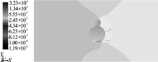
Fig.7 The distribution of pressure field

3.2Open-closed sequence of blade

The change of the blades at different time periods is studied based on one single blade. As shown in the figure, the angle in the theoretic opened and closed positions of the turbine is. According to the movement of the blade, a local coordinate system is built with the blade root as the origin. Assuming that the blade angle iswhen it is fully closed, the fully opened position of the blade is as shown in the figure, which is the vertical position formed by the connection from the blade vertex to the endpoint and in the flow direction. By determining the open-closed angle at point A through Ansys, the position of the blade can be obtained according to the azimuth angle.

Fig.8 Open-closed process of single blade

3.2.1 Open-closing sequence of single blade during rotation In Fig.8, the horizontal axis represents the rotating angle of the hydraulic turbine, while the vertical axis represents the opening angle of the blade. According to the figure, the maximum opening angle of the blade is approximately equal to. Due to the action of the connecting rods, the incident flow area of the blade is larger than that without the connecting rods, therefore a larger driving moment is generated. When the blade fully opens, the connection from the blade tip to the blade root is approximately in the flow direction and the driving moment at this moment reaches its maximum and the blade starts working. After the hydraulic turbine rotates to the position of aboutthe blade slowly closes and the next blade begins to enter into the operating state. After the turbine rotates to the position of about, the blade fully closes and then begins to enter into the start-up state after rotatingagain driven by other blades, and then after the hydraulic turbine rotates to the position of, the open-closed process of the blade is completed when the blade fully opens and enters into the operating state. The open-closed process of the blade should be fully symmetrical due to the presence of the connecting rods. Compared with those without the connecting rods, the blade opens earlier with a larger effective incident flow area and driving moment.

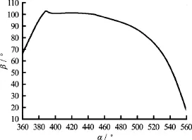
Fig.9 Fully opened and closed states of blade

Fig.10 Open-closed angles of three different blades at varying times

3.2.2 Variations of open-closed angle of different blades at different times during rotation In view of the presence of the connecting rod, thesix blades can be divided into 3 groups to study the angle variations of different blades at different times. Figure 8 shows the open-closed process of a single blade. Figure 9 indicates the fully opened and closed states of the blade. Figure 10 shows the open-closed angles of three different blades, each of which reaches the largest opening angle successively during rotation. When the blade represented by the first line fully opens, the blades represented by the second line and the third line are in the process of opening. After the blade represented by the second line fully opens, the blade presented by the first line begins entering into the closing state, and the blade presented by the third line is still in the process of opening. When the blade represented by the third line fully opens, the blades represented by the first line and the second line are in the process of closing. As the blade represented by the third line begins its closing state, the blade represented by the first line fully opens and the blade represented by the second line is still in the process of closing. Compared with those without the connecting rods, at least one pair of blades is working in the movement process of the hydraulic turbine, which guarantees the operation stability and improves the efficiency of the whole hydraulic turbine.

In the comparison of Fig.5 and Fig.10, the wave crest indicates that one certain blade fully opens and enters into the operating state, while the wave trough indicates that the blade begins to enter into the closed state. Simultaneously, the rotation velocity reaches the wave crest again and the next blade enters into the operating state. Thus, it can be observed that the rotation velocity shows a periodical movement after steady operating of the hydraulic turbine and within the whole process, six fluctuation periods are observed because each blade is going to obtain its largest opening angle successively. As the blade rotates, the incident flow area decreases gradually, so does the moment and then the rotation slows down. After moving to the position of, another blade enters into the operating state. At this moment, the driving moment of the blade reaches the maximum value, the acceleration changes abruptly and the velocity increases suddenly. Afterwards, the previous processes repeat with a periodic fluctuation.

3.3Variations of energy utilization coefficient and angular velocity with the resistance moment

The energy utilization coefficient of the hydraulic turbine is determined as the ratio of the output power to the kinetic energy of the ocean flow in the projective plane of hydraulic turbine’s impeller[21,22].

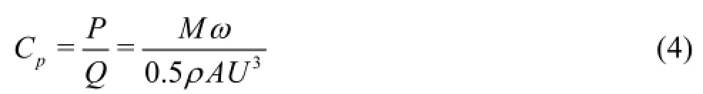
For comparing the results, the dimensionless velocity ratio is defined as follows in whichdenotes the velocity of the incident flow,the average angular velocity of the rotor, andthe valid radius of the hydraulic turbine, equal to the sum of the radiusof the wheel hub and the chord heightof the fully opened blade.

The tip-speed ratio inherently corresponds to the resistance moment in the simulation. With a fixed velocity of the incident flow and the hydraulic turbine,andare constant, i.e., the tip-speed ratio varies asand the average angular velocity is also constant with a constant resistance moment, indicating that there is a certain connection between the tip-speed ratio and the resistance moment.

According to the definition of the tip-speed ratio, with a constant hydraulic turbine size, the velocity of the incident flowis inversely related to the average angular velocityof the hydraulic turbine. With a given velocity of the incident flow, the resistance moments determine the variations of the energy utilization coefficient.

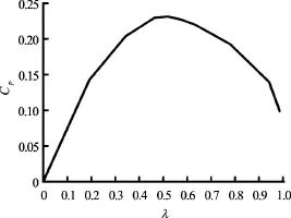
Fig.11 Variations of energy utilization coefficients with different tip-speed ratios

The variation trend of the average energy utilization coefficients of the hydraulic turbine under different tip-speed ratios is as shown in Fig.11, where, thehorizontal axis denotes the resistance moment and the vertical axis indicates the energy utilization coefficient. In this study, the energy utilization coefficient under different tip-speed ratios is obtained through Formula (5) based on the average angular velocity, which is derived from the hydraulic turbine velocity under different tip-speed ratios through numerical simulations. As shown in the figure, the energy utilization coefficient increases initially but decreases later on as the resistance moment increases. The average energy utilization coefficient maximizes as the tip-speed ratio lingers around 0.5, that is to say, the energy acquisition efficiency of the hydraulic turbine is the highest when the flow is 0.6 m/s and the tip-speed ratio is 0.5. As the tip-speed ratio reaches 1, the working efficiency of the hydraulic turbine decreases sharply and the energy utilization coefficient becomes less than 0.1. On the contrary, when the tip-speed ratio exceeds 1, the resistance moment is larger than the driving moment provided by the water flow, and the hydraulic turbine will not be able to run normally.

4. Conclusions

(1) From the turbine visualization tests, Yang et al.[19]obtained the open-closed sequences of the hydraulic turbine blade(without connecting rods), with the opening process starting at the position of about 90o, and finishing at the position of about 120o, while the closing process taking place between the positions of 180oand 360ohydraulic turbine rotates at the position of about 150o, the blade slowly closes, when the turbine rotates to the position of about 270o, the blade fully closes and finishes this process at the poaition of about 330o, then the blade slowly opens. Compared with those without connecting rods, the blades open earlier, the effective incident flow area increases and the blades close faster, therefore, the driving moment is larger. As there are always at least a pair of blades at the working state, the operation stability and the efficiency of the whole hydraulic turbine are improved.

(2) The maximum mean coefficient of the performance calculated for the blades is about 0.19 by Yang et al.[19]. With our numerical simulation, the maximum mean coefficient of the performance is about 0.23. So the power coefficient is higher than the turbines without connecting rods.

(3) As the resistance moment increases, the energy utilization coefficient of the hydraulic turbine increases first and then decreases later on. When the resistance moment increases to a constant value, the hydraulic turbine cannot operate normally. By an effective control over the resistance moment, the hydraulic turbine can maintain an optimal operating state.

[1] Chen J. H., Chiu F. C., Hsin C. Y. et al. Hydrodynamic consideration in ocean current turbine design [J].Journal of Hydrodynamics, 2016, 28(6):1037-1042.

[2] Shiono M., Suzuki K., Kiho S. Output characteristics of Darrieus water turbine with helical blades for tidal current generations [C].Proceedings of the Twelfth International Offshore and Polar Engineering Conference. Kitakyushu, Japan, 2002, 859-864.

[3] Khalid S. S., Zhang L., Zhang X. W. et al. Three-dimensional numerical simulation of a vertical axis tidal turbine using the two-way fluid structure interaction approach [J].Journal of Zhejiang University-SCIENCE A, 2013, 14(8): 574-582.

[4] Batten W. M. J., Bahaj A. S., Molland A. F. et al. Experimentally validated numerical method for the hydrodynamic design of horizontal axis tidal turbines [J].Ocean Engineering, 2007, 34(7): 1013-1020.

[5] Mao Z., Liu Q., Cui R. Discrete-time dynamical maximum power tracking control for a vertical axis water turbine with retractable blades [J].Discrete Dynamics in Nature and Society, 2016, 2016(3): 1-11.

[6] Lam W. H., Dai Y. M. Numerical study of straight-bladed Darrieus-type tidal turbine [J].Energy, 2009, 162(2): 67-76.

[7] Antheaume S., Maître T., Achard J. L. Hydraulic Darrieus turbines efficiency for free fluid flow conditions versus power farms conditions [J].Renewable Energy, 2008, 33(10): 2186-2198.

[8] Mohamed M. H. Performance investigation of H-rotor Darrieus turbine with new airfoil shapes [J].Energy, 2012, 47(1): 522-530.

[9] Maître T., Amet E., Pellone C. Modeling of the flow in a Darrieus water turbine: Wall grid refinement analysis and comparison with experiments [J].Renewable Energy, 2013, 51(2): 497-512.

[10] Qian Z. D., Yang J. D. Comparison of numerical simulation of pressure pulsation in Francis hydraulic turbine by different turbulence models[J].Journal of Hydroelectric Engineering, 2007, 26(6): 111-115.

[11] Ponta F., Dutt G. S. An improved vertical-axis watercurrent turbine incorporating a channelling device [J].Renewable energy, 2000, 20(2): 223-241.

[12] Ponta F. L., Jacovkis P. M. A vortex model for Darrieus turbine using finite element techniques [J].Renewable Energy, 2001, 24(1): 1-18.

[13] Li Y., Çalişal S. M. A discrete vortex method for simulating a stand-alone tidal-current turbine: Modeling and validation [J].Journal of Offshore Mechanics and Arctic Engineering, 2010, 132(3): 031102.

[14] Li Y., Çalişal S. M. Numerical analysis of the characteristics of vertical axis tidal current turbines [J].Renewable Energy, 2010, 35(2): 435-442.

[15] Hwang I. S., Yun H. L., Kim S. J. Optimization of cycloidal water turbine and the performance improvement by individual blade control [J].Applied Energy, 2009, 86(9): 1532-1540.

[16] Takata G., Katayama N., Miyaku M. et al. Study on power fluctuation characteristics of wind energy converters with fluctuating turbine torque [J].Electrical Engineering in Japan, 2005, 153(4): 1-11.

[17] Tian W., Song B., Mao Z. Conceptual design and numerical simulations of a vertical axis water turbine used for underwater mooring platforms [J].International Journalof Naval Architecture and Ocean Engineering, 2013, 5(4): 625-634.

[18] Myers L. E., Bahaj A. S. Experimental analysis of the flow field around horizontal axis tidal turbines by use of scale mesh disk rotor simulators [J].Ocean Engineering, 2010, 37(2-3): 218-227.

[19] Yang B., Lawn C. Fluid dynamic performance of a vertical axis turbine for tidal currents [J].Renewable Energy, 2011, 36(12): 3355-3366.

[20] Yang B., Lawn C. Three-dimensional effects on the performance of a vertical axis tidal turbine [J].Ocean Engineering, 2013, 58(2): 1-10.

[21] Torres F. R., Teixeira P. R. F., Didier E. Study of the turbine power output of an oscillating water column device by using a hydrodynamic-Aerodynamic coupled model [J].Ocean Engineering,2016, 125: 147-154.

[22] Dominguez F., Achard J. L., Zanette J. et al. Fast power output prediction for a single row of ducted cross-flow water turbines using a BEM-RANS approach [J].Renewable Energy,2015, 89: 658-670.

(Received January 3, 2016, Revised April 24, 2016)

* Project supported by the Science and Technology Development Project of Shandong Province of China (Grant No. 2014GGX103028).

Biography: Long-jing Li (1988-), Male, Ph. D.

Shen-jie Zhou,

E-mail: zhousj@sdu.edu.cn