Coupling methods of global climate models and regional climate models①

Wang Yuzhu (王玉柱), Jiang Jinrong, He Juanxiong

(*Institute of Remote Sensing and Digital Earth, Chinese Academy of Sciences, Beijing 100094, P.R.China) (**Computer Network Information Center, Chinese Academy of Sciences, Beijing 100190, P.R.China) (***Institute of Atmospheric Physics, Chinese Academy of Sciences, Beijing 100029, P.R.China)

Coupling methods of global climate models and regional climate models①

Wang Yuzhu (王玉柱)***, Jiang Jinrong②**, He Juanxiong***

(*Institute of Remote Sensing and Digital Earth, Chinese Academy of Sciences, Beijing 100094, P.R.China) (**Computer Network Information Center, Chinese Academy of Sciences, Beijing 100190, P.R.China) (***Institute of Atmospheric Physics, Chinese Academy of Sciences, Beijing 100029, P.R.China)

The future climate dynamical downscaling method is that output of general circulation models (GCMs) is employed to provide initial conditions, lateral boundary conditions, sea surface temperatures, and initial land surface conditions to regional climate models (RCMs). There are two methods of downscaling: offline coupling and online coupling. The two kinds of coupling methods are described in detail by coupling the Weather Research and Forecasting model (WRF) with the Institute of Atmospheric Physics of Chinese Academy of Sciences Atmospheric General Circulation Model Version 4.0 (IAP AGCM4.0) in the study. And the extreme precipitation event over Beijing on July 21 2012 is simulated by using the two coupling methods. Results show that online coupling method is of great value in improving the model simulation. Furthermore, the data exchange frequency of online coupling has some effect on simulation result.

coupling method, online coupling, climate model, performance evaluation, torrential rainfall

0 Introduction

General circulation models (GCMs) are used for forecasting weather, understanding climate and forecasting climate change. Atmospheric GCMs (AGCMs) numerically solve equations of physics (e.g., dynamics, thermodynamics, radiative transfer, etc.) and chemistry applied to the atmosphere and its constituent components, including greenhouse gases[1]. Due to huge computational cost[2,3], GCMs are usually used to simulate global climate at coarse spatial resolution. Now the resolution of GCMs which is below 100km is still too coarse to be directly used in regional climate impact studies. Therefore, global climate models with coarse resolution have no good simulation ability on a regional spatial scale[4,5], specifically for the topography, eddy processes and have some difficulty in parametrizing subgrid scale processes[6]. Regional climate models (RCMs) with high resolution can resolve more accurately regional variations in orography and land surface characteristics[5,7]. Downscaling of global model results has been used to address this issue by bridging the gap of scales between global and regional climate information[8-10]. That is, GCMs provide initial and lateral boundary conditions to RCMs[11,12]called offline downscaling or coupling. There are many previous studies on coupling regional climate models within global climate models[13,14].

Because of too long time interval (always several hours) of the GCM outputs, simulations of all the offline couplings suffer from some systematic biases in a way. Some bias correction methods such as correcting GCM outputs by observations have been used for improving the simulation of regional climate downscaling. Meanwhile online coupling RCMs with GCMs has been used at the forefront of model development to decrease time interval of outputs used for lateral boundary conditions. The data exchange frequency of online coupling is much higher than that of offline coupling, so the data exchange frequency can be increased to improve the simulation results. The Institute of Atmospheric Physics (IAP) of Chinese Academy of Sciences (CAS) has designed and developed a new fully coupled climate system model (Chinese Academy of Sciences-Earth System Model, CAS-ESM)[15]. The CAS-ESM system achieves the online coupling of the Institute of Atmospheric Physics of Chinese Academy of Sciences Atmospheric General Circulation Model version 4.0 (IAP AGCM4.0) and Weather Research and Forecasting model (WRF) by the coupler.

Extreme weather and climate events have major impacts on the society, economy and environment. Torrential rainfall is one of the major weather disasters in China. Affected by the summer monsoon, the summer rainfall areas are mainly in southern China, Jianghuai district and northern China. The heavy rain period of northern China with highly intense precipitation mostly occurs in July and August of the summer. Northern China, where China’s capital Beijing is, has varied and complicated topography and dense population. Therefore, if torrential rainfall occurs, it would lead to huge economic loss and endanger people’s lives and property. The heaviest rainfall over 61 years hit Beijing on 21-22 July 2012[16]. The torrential rainfall caused landslides and floods, killed 79 people, and caused direct economic losses of nearly ＄2 billion[17].

Many papers usually describe some coupling application of GCMs and RCMs, however, there are no researches on their comparison and implementation details of offline and online couplings. Therefore, the coupling methods and implementation details of GCM and RCM are studied. During assessing simulation ability of offline and online couplings, the study chooses the torrential rainfall event in Beijing as the experiment case. For the offline coupling, the IAP AGCM4.0 model is used to drive WRF. And the CAS-ESM is employed to evaluate the online coupling of IAP AGCM4.0 and WRF.

The paper is organized as follows. Section 1 mainly introduces the global model IAP AGCM4.0 and regional model WRF. Section 2 describes two kinds of coupling methods and experiment setup. Section 3 analyses and discusses the simulation results of the four experiments. The last Section contains a summary.

1 Models

1.1 Atmospheric global circulation model

An AGCM usually consists of the “dynamics” (dynamical core) and the “physics” (physical process). The dynamical core calculates atmospheric flow and solves the hydrodynamic equations of atmosphere. Then, the physical process parameterizations for subgrid phenomena such as long- and short-wave radiation, moist process, and gravity wave drag[18]. The total frame diagram of an AGCM is presented in Fig.1.

In the study, the GCM model used is the IAP AGCM4.0 model which uses the Community Atmosphere Model version 3.1 physics package of the National Center for Atmospheric Research is developed by IAP[19]. For the IAP AGCM4.0, the T42 spectral dynamical core with a horizontal resolution of 1.4° latitude by 1.4° longitude and 26 levels in the vertical direction is employed. The initial conditions and lateral boundary conditions are from National Centers for Environmental Prediction (NCEP) re-analysis data.

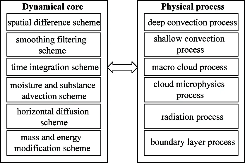
Fig.1 Total frame diagram of an AGCM

1.2 Regional climate model

The regional climate model is the Advanced Research WRF (ARW) Version 3.2. WRF is often used to forecast weather and simulate climate. The integration domain which covers all of Beijing has 401 grids along the East-West direction and 281 grids along the North-South direction, with the center at 40°N, 116°E. In the WRF, the grid spacing is 30km and vertical direction is 31 sigma levels with the model top at 50hPa. The time step of the WRF is set to 50s. The WRF physics use Rapid Radiation Transfer Model (RRTM) long-wave radiation scheme, Dudhia short-wave radiation scheme, Yonsei University planetary boundary layer scheme, Kain-Fritsch cumulus scheme, Lin microphysics scheme, Monin-Obukuhov surface layer scheme and Noah land surface scheme. The initial conditions and lateral boundary conditions are from NCEP re-analysis data or IAP AGCM4.0 output.

1.3 CAS-ESM model

The CAS-ESM is developed from the Community Earth System Model version 1.0. Composed of six separate models simultaneously simulating the Earth’s atmosphere, ocean, land, land-ice, sea-ice and atmospheric chemistry, plus one central coupler component, the CAS-ESM allows researchers to conduct fundamental research for the Earth’s climate states. In the CAS-ESM system, the atmosphere component model used is the IAP AGCM4.0, the ocean component model is the LASG/IAP Climate System Ocean Model (LICOM) version 2.0 developed by the State Key Laboratory of Numerical Modeling for Atmospheric Sciences and Geophysical Fluid Dynamics (LASG) of the IAP, the land component model is the Common Land Model (CoLM) developed by Beijing Normal University, the sea-ice component model is the CICE version 4, the land-ice component model is the GLC and the atmospheric chemical component model is the Global Environmental Atmospheric Transport Model (GEATM) developed by IAP.

Besides the six separate model components, WRF is also put into the CAS-ESM modeling system. Here, WRF is considered as a part of the IAP AGCM4.0 source code. Meanwhile, the four computation models (geogrid, metgrid, real, integration) of WRF are integrated together in order to make the IAP AGCM4.0 drive the WRF online. That means that the IAP AGCM4.0 provides the initial conditions, lateral boundary conditions, surface temperature, and soil moisture online to the WRF. The data exchange between the IAP AGCM4.0 and WRF is achieved through the CAS-ESM Coupler version 7 (CPL7). The model structure of the CAS-ESM system is presented in Fig.2.

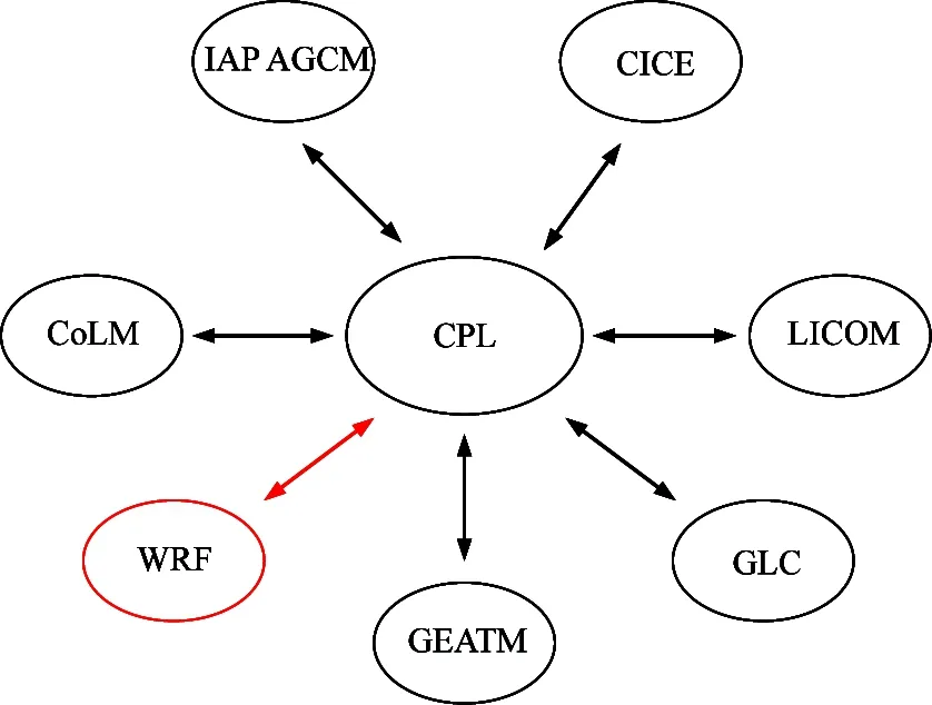
Fig.2 Model structure of the CAS-ESM

In the study, data ocean model, the prescribed sea-ice model, active land model Community Land Model (CLM) and atmospheric model IAP AGCM4.0 in the CAS-ESM are employed to only evaluate the online coupling of the IAP AGCM4.0 and WRF.

2 Coupling methods and experiment setup

2.1 Offline coupling

The process of offline coupling of GCMs and RCMs is quite simple. A GCM is executed at first, then the output of GCM is used to drive a RCM. However, during the whole offline coupling process, the researchers have to manually perform these operations in turn and implement some data conversion.

Fig.3 shows the flow chart of the offline coupling of the IAP AGCM4.0 and WRF. The fnl2cam.ncl script is used to read data from the NCEP final analysis (NCEP-FNL) data with GRIB1 format and produce the initial data file for the IAP AGCM4.0. The CAM2WRF software package is used to convert the outputs of the IAP AGCM4.0 to the intermediary format file needed by the WRF Preprocessing System (WPS).

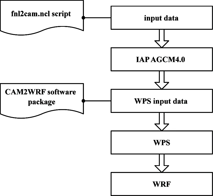
Fig.3 Flow chart of the offline coupling of the IAP AGCM4.0 and WRF

2.2 Online coupling

The aim to online coupling is that a GCM can drive a RCM in real time for many times. Generally, online coupling is achieved by the coupler. Sometimes, the source code of a RCM is considered as a part of a GCM. During the whole online coupling process, the researchers don’t have to manually perform these operations. In online coupling, the time interval of data exchange between GCMs and RCMs could be a few minutes or a few seconds. And yet, the one in offline coupling is 3 hours or 6 hours. Therefore, online coupling can achieve higher data exchange frequency.

Fig.4 describes the flow chart of time integration of the WRF in the CAS-ESM system, where the coupling time interval between the IAP AGCM4.0 and CPL7 is atm_cpl_dt, and the one between the WRF and CPL7 is wrf_cpl_dt. The wrf_cpl_dt can be set to the IAP AGCM4.0 time step or an integral multiple of the IAP AGCM4.0 and WRF time steps. When the CPL7 sends the data to the WRF at each time step of data exchange, the WRF updates its lateral boundary data set and other data information[20]. The fields that the WRF receives from the CPL7 are listed in Table 1.

Table 1 Variables received by the WRF from the CPL7

Fig.4 Flow chart of time integration of the WRF in the CAS-ESM

2.3 Experiment schemes

To simulate the extreme precipitation event over Beijing on 21 July 2012 (00:00 universal coordinated time (UTC) 21 July 2012 to 00:00 UTC 22 July 2012), the paper sets four numerical experiments.

(1) The first experiment only uses the WRF to simulate the event. The 6-hour NCEP-FNL data (from 00:00 UTC 21 July 2012 to 00:00 UTC 22 July 2012) is employed to drive the WRF.

(2) The second experiment is an offline coupling testing using the IAP AGCM4.0 and WRF. First, the 6-hour NCEP-FNL data at 00:00 UTC 21 July 2012 is employed to drive the IAP AGCM4.0. Then the output of the IAP AGCM4.0 is used to drive the WRF.

(3) The third experiment is an online coupling testing using the CAS-ESM, where the IAP AGCM4.0 is also driven by the 6-hour NCEP-FNL data at 00:00 UTC 21 July 2012 and the output of the IAP AGCM4.0 is equally used to force the WRF. The time interval of the data exchange between the WRF and CPL7 is 1 hour. That is, the frequency of data exchange is 24 times per day.

(4) The fourth experiment is also an online coupling testing with 1/3 hour time interval. It means that the frequency of data exchange is 72 times per day.

The first and second experiments are offline coupling, and the third and fourth experiments are offline coupling.

2.4 Data

The observation data including the site precipitation data based on the MICAPS system are provided by the China Meteorological Administration.

In the first and second experiments, the 6-hour NCEP-FNL data at 1°×1° resolution is used to provide initial conditions for the IAP AGCM4.0 and WRF model. The NCEP-FNL data which corrects GCM outputs by observations is one of the datasets used for real time simulations.

In the third and fourth experiments, the initial conditions for the IAP AGCM4.0 are generated by interpolating the NCEP-FNL 1°×1° data to the T42 Gaussian grids by using the first-order area-weighted mapping. The CLM is spun up using the atmosphere data model in the CSA-ESM (DATM7) and the surface forcing of Qian et al[21]for 10 years up to the starting date and time of the experiment. The sea surface temperature and sea ice data are from the National Oceanic and Atmospheric Administration (NOAA) Optimum Interpolation sea surface temperature V2 data set with weekly temporal resolution and 1°×1° spatial resolution.

3 Results and discussion

The validation and comparison of the four experiment results are based on the observations. The observations of the daily-accumulated rainfall from 00:00 UTC on 21 July 2012 to 00:00 UTC on 22 July 2012 are shown in Fig.5. The observations indicate that the 24h rainfall of the whole Beijing city is more than 100mm and the intensive precipitation area whose center is Beijing extends from southwest of Beijing to its northeast.

Fig.5 Accumulated 24 hours observation precipitation

The daily-accumulated rainfall of all the four simulations is smaller than the observations. However, the rainbands of the four simulations are different. As shown in Fig.6, the first experiment can reproduce the observed precipitation distribution tendency. Comparing with the observations the precipitation center is to the north. Fig.7 shows the daily-accumulated rainfall in the second experiment. There are two rainbands with accumulated rainfall of more than 100mm, but there is only a main rainband in the observations. Fig.8 and Fig.9 show the daily-accumulated rainfall in the third and fourth experiments. Both of the rainbands become one and the rainbands are to the south comparing with the first experiment although the precipitation center is still to the north comparing with the observations. The results show that the online coupling of the IAP AGCM4.0 and WRF can produce better simulation than the offline coupling.

According to comparing Fig.8 with Fig.9, it is found that the simulation results of the two online couplings are similar, sometimes even better than driving the WRF with NCEP-FNL reanalysis data. However, the data exchange frequency of the online coupling has also some effect on the simulation result and the online

Fig.6 Rainfall in the first experiment

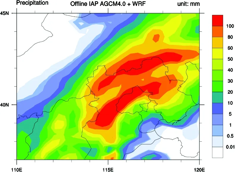
Fig.7 Rainfall in the second experiment

Fig.8 Rainfall in the third experiment

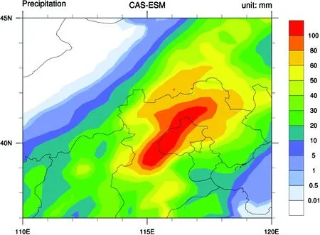
Fig.9 Rainfall in the fourth experiment

coupling with higher data exchange frequency does not necessarily produce better result.

4 Conclusions

The study introduces offline and online coupling methods of GCMs and RCMs at first, then achieves the offline and online coupling of the IAP AGCM4.0 and WRF. According to employing the offline and online coupling to simulate the extreme precipitation event over Beijing on 21 July 2012, the study draws a conclusion that the online coupling simulates better than the offline coupling. In addition, the data exchange frequency of the online coupling has also some effect on the simulation result. In a word, it is quite meaningful to continue to study and utilize the online coupling of GCMs and RCMs for climate simulation in the future.

[1] Mann M, Gaudet B. General circulation models. https://www.e-education.psu.edu/meteo469/node/140:The Pennsylvania State University, 2015

[2] Taylor K E, Stouffer R J, Meehl G A. An overview of CMIP5 and the experiment design. Bulletin of the American Meteorological Society, 2012, 93(4): 485-498

[3] Montoya M, Griesel A, Levermann A, et al. The earth system model of intermediate complexity CLIMBER-3α. Part I: description and performance for present-day conditions. Climate Dynamics, 2005, 25: 237-263

[4] Giorgi F. Perspectives for regional earth system modeling. Global and Planetary Change, 1995, 10(1): 23-42

[5] Giorgi F. Simulation of regional climate using a limited area model nested in a general circulation model. Journal of Climate, 1990, 3: 941-963

[6] Duffy P B, Govindasamy B, Iorio J P, et al. High-resolution simulations of global climate, part 1: present climate. Climate Dynamics, 2003, 21: 371-390

[7] Anthes R A, Kuo Y H, Low-Nam S, et al. Estimation of skill and uncertainty in regional numerical models. Quarterly Journal of the Royal Meteorological Society, 1989, 115: 763-806

[8] Seth A, Rauscher S A, Camargo S J, et al. RegCM3 regional climatologies for South America using reanalysis and ECHAM global model driving fields. Climate Dynamics, 2007, 28: 461-480

[9] Giorgi F, Hewitson B, Christensen J, et al. Regional Climate Information—Evaluation and Projections. Cambridge: Cambridge University Press, 2001. 583-638

[10] Bukovsky M S, Karoly D J. A regional modeling study of climate change impacts on warm-season precipitation in the Central United States. Journal of Climate, 2011, 24: 1985-2002

[11] Cocke S, LaRow T E. Seasonal predictions using a regional spectral model embedded within a coupled ocean-atmosphere model. Monthly Weather Review, 2000, 128: 689-708

[12] Liang X Z, Pan J, Zhu J, et al. Regional climate model downscaling of the U.S. summer climate and future change. Journal of Geophysical Research: Atmospheres, 2006, 111 (D10)

[13] Giorgi F, Brodeur C S, Bates G T. Regional climate change scenarios over the United States produced with a nested regional climate model: Spatial and seasonal characteristics. Journal of Climate, 1994, 7: 375-399

[14] Dickinson R E, Errico R M, Giorgi F, et al. A regional climate model for the western United States. Climatic Change, 1989, 15: 383-422

[15] Dong X, Su T H, Wang J, et al. Decadal Variation of the Aleutian Low-Icelandic Low Seesaw Simulated by a Climate System Model (CAS-ESM-C). Atmospheric and Oceanic Science Letters, 2014, 7 (2): 110-114

[16] Liu J, Wang S Y. Analysis of human vulnerability to the extreme rainfall event on 21-22 July 2012 in Beijing, China. Natural Hazards and Earth System Sciences, 2013, 13(11): 2911-2926

[17] Zhang D L, Lin Y, Zhao P, et al. The Beijing extreme rainfall of 21 July 2012: “Right results” but for wrong reasons. Geophysical Research Letters, 2013, 40(7): 1426-1431

[18] Mirin A A, Sawyer W B. A scalable implementation of a finite-volume dynamical core in the community atmosphere model. International Journal of High Performance Computing Applications, 2005, 19: 203-212

[19] Zhang H, Zhang M, Zeng Q. Sensitivity of Simulated Climate to two atmospheric models: interpretation of differences between dry Models and moist models. Monthly Weather Review, 2013, 14: 1558-1576

[20] He J, Zhang M, Lin W, et al. The WRF nested within the CESM: Simulations of a midlatitude cyclone over the Southern Great Plains. Journal of Advances in Modeling Earth Systems, 2013, 5: 611-622

[21] Qian T, Dai A, Trenberth K E, et al. Simulation of global land surface conditions from 1948 to 2004. Part I: Forcing data and evaluations. Journal of Hydrometeorology, 2006, 7(5): 953-975

Wang Yuzhu, born in 1988. He received his Ph.D degree from University of Chinese Academy of Sciences in 2015. He also received his B.S. degree from Chongqing University in 2010. Now he is a postdoctor researcher at Institute of Remote Sensing and Digital Earth, Chinese Academy of Sciences (CAS), Beijing, China. His research interests include parallel algorithm, high performance geo-computing, and development of earth system model.

10.3772/j.issn.1006-6748.2017.01.013

①Supported by the National Natural Science Foundation of China (No. 61602477), China Postdoctoral Science Foundation (No. 2016M601158), and National Key Research and Development Program of China (No. 2016YFB0200804).

②To whom correspondence should be addressed. E-mail: jjr@sccas.cn Received on Dec. 23， 2015