A review of some methodological developments on fullwaveform inversion tackled in the SEISCOPE group
2017-03-15RomainBROSSIERLudovicTIVIERJeanVIRIEUXYANGPengliangZHOUWei
Romain BROSSIER,Ludovic MÉTIVIER,Jean VIRIEUX,YANG Pengliang,ZHOU Wei
(1.Univ.Grenoble Alpes,ISTerre,Grenoble,France;2.Univ.Grenoble Alpes,CNRS,LJK,Grenoble,France)
A review of some methodological developments on fullwaveform inversion tackled in the SEISCOPE group
Romain BROSSIER1,2,Ludovic MÉTIVIER1,2,Jean VIRIEUX1,2,YANG Pengliang1,2,ZHOU Wei1,2
(1.Univ.Grenoble Alpes,ISTerre,Grenoble,France;2.Univ.Grenoble Alpes,CNRS,LJK,Grenoble,France)
Full waveform inversion (FWI) is a data-fitting inverse problem aiming to delineate high-resolution quantitative images of the Earth.While its basic principle has been proposed in the eighties,the approach has been significantly developed and applied to 2D and 3D problems at various scales for the last fifteen years.Despite these successes,FWI is still facing some issues for applications in complex geological setups because of some lack of robustness and automatic workflow,while being computationally intensive.In this paper,after a short review of the basic FWI formulation and analysis of the FWI gradient,three recent methodological developments performed in the frame of the SEISCOPE project are presented.First,an algorithmic development is presented as a low-memory and computationally efficient approach for building the time-domain FWI gradient in 3D viscous media.Second,a reformulation of FWI is performed to handle reflections in their tomography regime while still using the diving waves,leading to the joint full waveform inversion (JFWI) approach.Finally,an optimal transport approach is proposed as an alternative to the classical difference-based misfit for mitigating the cycle-skipping issue.
FWI,attenuation,JFWI,checkpoint,cycle-skipping
1 Introduction
Full waveform inversion (FWI) is a data-fitting procedure that aims to reconstruct high-resolution models of the Earth’s subsurface from the full information contained in seismic data.Proposed almost simultaneously by LAILLY[1]and TARANTOLA[2],FWI has been proposed to reconstruct quantitative estimation of the rock properties based on the resolution of a data-fitting inverse problem.While the method has been proposed more than thirty years ago,the number of the FWI successes has dramatically increased for the last fifteen years thanks to the advances of the computer capability and data acquisition.Indeed,when the FWI was proposed in the eighties,the first applications faced two main limitations[3-12].The first issue was the computational cost:in the eighties,computing the full wave-equation solutions in heterogeneous media with numerical methods such as finite-differences or finite-elements was quite expensive for multiple sources even in two-dimensional geometries.More importantly,FWI was mainly applied to surface seismic data,mostly dominated by reflections as streamer lengths were only a few kilometers and without low frequency content.This led to the inability of FWI to provide a broadband reconstruction of the Earth structure[9]and the method was almost unusable.
In the nineties,FWI rebirthed,pushed by the work of PROF.G.PRATT who smartly combined appropriate data type (cross-well data),hierarchical multiscale approach to mitigate the non-linearity and efficient frequency-domain formulation.PRATT’s work showed that if appropriate data and hierarchy were used,and even if computationally more intensive that ray-based approaches,the FWI concept was able to provide very promising results[13-18].Meanwhile,the multiscale approach was also developed to mitigate the nonlinearity of surface-based time-domain FWI by BUNKS et al[19].Using successive bandpass filtered version of the data.This understanding of the necessity to combine frequency hierarchy and different types of seismic arrivals (reflections,diffractions and transmissions) led the community to apply FWI to 2D geometries with surface-based data including long offsets[20-24],before extending the approaches to 3D problems for both controlled-source exploration and earthquake seismology[25-35].
Today,academic groups apply FWI to seismic data at various scales and the industry has included FWI in their velocity model building workflows for many of their depth imaging projects,leading to an impressive number of FWI applications.However,many problems still hold and prevent applying FWI for all targets.Among the issues of FWI,we can enumerate the computational cost of the approach;the non-linearity associated with the cycle-skipping issue and the quality of the initial model;the problems of multiparameter reconstructions and their trade-off;the source wavelet estimation;the issue of imaging at depths not sampled by diving waves[36].In this paper,we will first review and analyze basics of the FWI formulation and its associated gradient.Indeed,many issues of FWI can be anticipated from an analysis of the FWI gradient.Then,we will present three methodological developments performed recently in the SEISCOPE project:design of an optimal scheme for time-domain FWI formulation,Reflected-wave Waveform Inversion (RWI) and Joint Full Waveform Inversion (JFWI),and alternative misfit function based on the Optimal Transport distance.
2 Theory of classical FWI
The FWI is an inverse problem aiming to retrieve the parameters of a wave-equation partial differential equation (PDE) by optimizing the fit between observed and synthetic data.Let us definedobsthe observed data vector for one seismic source and a set of receivers positions,and the associated synthetic data vectordcal.Classically,FWI aims to minimize the waveform misfit [dobs-dcal(m)] by adjusting the parameters of the vectormof the wave-equation.Note that the observed data can be considered either in the time-domain (t) or in the frequency-domain (ω,the angular frequency).The classical FWI misfit-function relies on theL2norm of the data difference vector written as[2,36]
(1)
where ∑srcisthesumoversourcesand∑t,wisthesumovertimesamplesorfrequenciesdependingontheformulation,andsuperscript†standsfortheadjoint:transposeforrealoperatorsandconjugatetransposeforcomplexoperators.
Thesyntheticdatadcalat receiver positions are generally extracted from a wavefielduwith the extraction/sampling equation
(2)
whileu(m) satisfies a wave-equation PDE solved numerically with a volumetric method as finite-differences or finite-elements (the forward problem),andRis the sampling operator.Let us consider a generic discrete second order time-domain wave-equation
(3)
with appropriate initial and boundary conditions,or its equivalent form in the frequency domain
(4)
with appropriate boundary condition,whereM,CandKare the mass,viscous and stiffness matrices,respectively,andfis the source term.
For the sake of simplicity and compactness,equations (3) and (4) can be written in the form
(5)
where the time or frequency dependency has been dropped out for generality.Note that time-domain formulations rely generally on explicit time-marching approaches,while frequency-domain formulations rely on resolutions of linear systems for each frequency.
When considering FWI for realistic size problems,the size of the parameter and the data spaces,combined with the computational cost of the forward problem,leads naturally to local minimization schemes for equation (1).Local optimizations rely,at least,on the first-derivative,namely the gradient,of the misfit function with respect to the parametersm.The FWI gradient expression can be obtained through the Fréchet derivative matrix,referred to as the scattering-integral approach,leading to interesting physical understanding[16],or through the adjoint-state formalism[37]which provides a systematic formulation[38-39].Here we mainly focus on the equations of interest for the implementation and the understanding,while a complete mathematical development is omitted.After proper mathematical developments,the FWI gradient,for one seismic source,writes
(6)
where the notation <.|.>(t,ω) stands for the scalar product over time or frequency,uis the state field andλ1is the adjoint-state field.The state field requires to satisfy the forward problem equation (5),while the adjoint-state field is the solution of the adjoint state equation
(7)
When using theL2norm of the data difference as misfit function,We can note that the adjoint-source termR†(dobs-dcal) corresponds to the data residuals spatially located at the receiver positions.
Equations (5),(6) and (7) show that the FWI gradient is computed through a zero-lag correlation of two wavefields,one computed with the wave-equation operatorF(m) and the other with its adjointF(m)†.
More in details,for a time-domain FWI,the gradient writes[2,39]
(8)
where the state field u(t)is subjected to initial condition and the adjointstate λ1(t)is subjected to final condition (or an initial condition after a change of variable=T-t).
In the frequency-domain,the gradient writes[16,39]
(9)
Once the FWI gradient is computed,the descent direction Δmkcan be used to update the parameter through
(10)
wherekis the iteration number,αkis the steplength in the descent direction Δmk.This descent direction can be obtained through various optimization algorithms,from the simplest steepest descent (Δm=-∂mC) to more evolved preconditioned conjugate gradient or quasi-Newton (as L-BFGS)[40].
3 Analysis of the FWI gradient and identification of FWI issues
In order to identify some of the difficulties associated to FWI,let us analyse the expression of the frequency-domain FWI gradient at positionxifor the parametermi.This can be written as
(11)
when considering that ∂mF(m) is a null matrix everywhere except at position (i,i) and only a single frequency and single source.This simple expression can be analysed in the frame of diffraction tomography[41-42],considering a single source/receiver pair,source and receiver far from the diffraction pointxi,an homogeneous background medium and monochromatic plane waves for the incident and adjoint fields.We can therefore write


(14)

(15)

Figure 1 Scheme of gradient building with source and receiver plane waves from angles φs and φr
withφ=φs+φrand the moduluskis related to the local wavelength (λ=c0/f,withc0the velocity andfthe frequency) and the scattering angle (θ) by
(16)
From equation (16) and the associated graphic representation in Figure 2,we can see that both the frequency and acquisition geometry (acting on incidence angles) jointly affect the reconstructed wavenumber spectrum.For example,low wavenumbers can be obtained thanks to low frequencies data and wide aperture angles (θ≈π).
This analysis of the FWI gradient resolution,the adjoint-state equation (7) and the time-domain FWI gradient formula (8) allow to identify several potential issues we have worked on for the past years,and which will be further developed in the following sections:algorithmic issue associated to the time-domain FWI gradient,extraction of information from reflected waves at depth and the definition of the FWI misfit function.
4 Optimal algorithm to build time-domain FWI gradient
By analyzing the time-domain FWI gradient (8) and the associated fields equations (5) and (7),an algorithmic issue appears.Indeed,the FWI gradient is computed as a zero-lag crosscorrelation between a forward-time propagative fielduand a backward-time propagativeλ1.The backward-time propagativeλ1is obtained after an appropriate change of variable on time,to recast the adjoint field computation as an initial value problem to be computed backward in time with the adjoint of the forward operator.This zero-lag cross-correlation means that the two wavefields are not simultaneously available when considering usual explicit time-stepping.For realistic 3D problems,it is not feasible to store the incident fielduin core memory and accessing the incident field during the adjoint field computation to perform this gradient building step (also the same as cross-correlation imaging condition in reverse time migration (RTM)).Three main classes of method may be identified to perform this key step:
1) One may store in memory or on disk the incident wavefield when performing the incident modeling,and accessing it at each time step when computing the adjoint wave-field.This approach generally requires significant I/Os and requires data compression[43-44]or hardware-oriented strategies[45].
2) Another option is the checkpointing strategy,which recomputes the incident field forward in time inside a time window started with saved snapshots (checkpoints) at specific times[46-50].Each time step has to be recomputed several times from checkpoints,leading to a recomputation ratio (the total number of computed time-steps of the incident field,divided by the number of time-steps for one single incident simulation) much higher than two

Figure 2 Scheme of gradient building and associated resolution depending on the frequency and source/receiver waves relative incidence angles
when moderate memory resources are available.
3) The last approach is the wavefield reconstruction by reverse propagation:exploiting the reversibility of the wave-equation (in non-dissipative media),the incident wavefield can be almost perfectly recomputed backward in time from the final snapshot and boundary conditions at each time-step[51-57].This approach requires a recomputation ratio of two.
The recomputation ratio of factor two for the last approach is quite appealing for FWI and RTM problems but leads to algorithmic issues we detail in the following.
Memory saving thanks to compression
The first issue is the memory cost to store the boundary values of the wavefields at each time step.Considering an×n×n3D simulation box withnttime steps,the memory cost scales toan2nt,withaa constant depending on the numerical method and the wave-equation used.For some applications,this boundary storage can still be quite large.A compression approach has been investigated in YANG et al[58].relying on decimation plus interpolation on the time-history of the saved boundaries:during the forward computation of the incident field,the boundary storage is decimated down to Nyquist sampling.During the backward simulation,the missing values are reconstructed by interpolation using the saved down-sampled values.
The Courant-Friedrichs-Lewy (CFL) condition is a fundamental criterion to determine temporal sampling to achieve stable wavefield extrapolation.Let us consider for example a staggered grid finite-difference scheme[59-60],the CFL condition writes
(17)
whereaiare the coefficients of the staggered grid finite difference (FD) of order 2J,Δtand Δxare the temporal and spatial interval after discretization;vmaxis the maximum velocity;Dis the number of dimensions.Considering for example a typical 3D case with 4-th order spatial FD discretization,we have
(18)
Based on the usual discretization rule of 5 grid points per wavelength,we end up with
(19)
yielding
(20)
in whichfmaxandvminare maximum frequency of the signal and minimum velocity of the media,respectively.
However,the Dirichlet boundary condition used to inject the boundary sequence in time for the backward time simulation of the incident field is essentially determined by Nyquist sampling principle,rather than the time interval given by CFL.Nyquist sampling tells us that a signal can be perfectly reconstructed if we satisfy the condition
(21)
It implies that the boundary saving process could be loosely downsampled with a ratiorwithout any information loss,where the ratio is
Based on this result,a significant memory saving can be achieved by downsampling the boundary value up to Nyquist sampling:the higher the velocity contrast is,the higher the compression will be,allowing typical saving of factor 15 for realistic acoustic modeling and up to 50 for elastic modeling.
The missing values are then reconstructed on the fly during the backward-time simulation of the incident field.In YANG et al[58].three boundary interpolation techniques,namely the discrete Fourier transform (DFT) interpolation,Kaiser windowed cardinal sine interpolation and Lagrange polynomial interpolation,have been assessed and show negligible error in the reconstructed wavefield.
Tackling attenuation issue
The second issue of wavefield reconstruction by reverse propagation is the requirement to rely on a reversible wave-equation.When considering realistic attenuation models,this assumption generally breaks down.Indeed,the forward-time wavefield is damped through the use of memory variables[61-62]relying on exponential decaying function e-wlΔtat each time step Δtfor the mechanism whose reference frequency iswl.When considering backward time simulation,the exponential function has,however,to be considered as the growing function ewlΔtwhich causes accumulation of growing round-off error leading to instability for most of realistic attenuation models.In YANG et al[63].we designed a new algorithm which optimally combines the wavefield reconstruction by reverse propagation and the optimal checkpointing strategy,giving the “Checkpointing assisted reverse-forward simulation” (CARFS).This approach relies on an indicator of the stability of reverse propagation,through the global instantaneous energy.This measure is a good candidate to monitor the stability of the simulation,thanks to its sensitivity to variations of all wavefield components.During the forward-time simulation,the global instantaneous energy is computed and stored for each time-step (one scalar value for the whole 3D volume at each time step).Then during the simulation of the adjoint field,the leading idea of the CARFS algorithm is to use,as a default setting,the reverse propagation for the incident field even when attenuation is considered while monitoring the energy of the computation.At any given time step,if the energy of the backward simulation deviates from the monitored one computed during the forward simulation,from a user-defined threshold,the reverse propagation is temporarily stopped and checkpointing is used starting from the closest snapshot prior to current state to redo some forward time stepping in order to reinitialize the reverse propagation.In practice,at most of the time steps,the round-off errors do not create instabilities and the incident field can be computed backward in time.Once instability is detected,the checkpoints are used to reinitialize the wavefield through forward simulation.The algorithm has proved to be always more efficient than checkpointing-based approaches,providing an alternative of choice for time-domain FWI gradient.This workflow is described in more details in the algorithm 1.
Figure 3 is showing the 2D visco-acoustic Valhall model,inspired by the geology of the Valhall field,North Sea.The model exhibits some gas layer in the sediment,creating low velocity and low quality-factor value.Below,an anticlinal is the top layer of the oil reservoir.To compute wave propagation up to 80Hz in this model with finite-differences method,a 1671×2813 grid is used with grid spacing Δx=Δz=3.125m.Table 1 is showing the performance of the CARFS algorithm for different maximum frequencies.As the attenuation effects on the wavefield are directly linked to the frequency content of the simulation,we can see that the higher the frequency is,the higher the recomputation ratio of CARFS is.As the wavefield is more damped at higher frequency,more re-initializations with checkpointing are required.However,it can be seen that CARFS is always cheaper than checkpointing,whatever is the frequency content.This observation comes from the fact that,even in the worst case,CARFS would simply converges toward checkpointing and can not become more expensive.Figure 4 is showing the monitoring of the global instantaneous energy (panel (a)) and one seismic trace (panel (b)) at a randomly selected point in the model during the forward and backward computations at 80Hz.Also,the associated residual trace (panel (c)) is showing a negligible error for imaging or inversion purposes.
Therefore,CARFS provides an automatic alternative of choice for recomputing the incident field required for FWI and RTM applications.

Figure 3 The 2D Valhall synthetic modela the velocity; b the density; c the quality factor Q

Figure 4 Performance of CARFS coupled with the decimation plus interpolation approach on the boundaries,on the 2D synthetic visco-acoustic Valhall model.(a) The total instantaneous energy measure,(b) randomly extracted seismic traces and (c) trace error during the forward simulation and backward computation for fmax=80Hz[63]

1Distributecheckpointss0,…,sc-1intimefollowingthebinomiallawofoptimalcheckpointing;2forn=0,…,N-1do3computethewavefieldstateforwardintime:Fn:wn→wn+1andrecordthetotalenergyEn+1fforwn+1;4storetheboundaryofwn+1atdecimatedtemporalloca-tionsaccordingtoNyquistsampling[58];5ifn∈s0,…,sc-1thenstorethesnapshotwn+1;6end7forn=N-1,…,0do8findtheclosestcheckpointsipriortocurrenttimeleveln(si≤n
5 Reflection-oriented waveform inversion and joint full waveform inversion
From equation (16),one issue is appearing for reflected waves at depth:when considering deep targets sampled by reflected-waves-only,as the limited available offsets prevent the recording of diving waves,the range of scattering angles is narrower than for shallow targets sampled by reflections and transmissions.This limited range of angles and their small values lead naturally to the reconstruction of high wavenumber components.At such depths,the lack of large scattering angles prevents the reconstruction of low wavenumbers with the common available frequency content,leading to a gap in the wavenumber spectrum (c.f.figure 1.4-3 from CLAERBOUT[64],also the same observation was done by JANNANE et al[9].
This idea of exploiting reflections for building the low-wavenumber components of the velocity model,inspired by the work of CHAVENT et al[65];CHAVENT[66];CLÉMENT et al[67].on migration-based travel time inversion (MBTT),has been recently explored in the frame of waveform inversion giving the reflection-oriented waveform inversion (RWI)[68-74].
Relying on the same scale separation assumption than the one used in most of classical reflection-based tomography methods and migration-based ve-
Table 1 CARFS performances:number of time stepping and recomputation ratio in CARFS for varying highest reference frequency in the 2D visco-acoustic Valhall model of figure 3.fmaxis the maximum frequency of the simulation,N′ is the total number of time steps required to achieve the forward-time simulation of the incident field and its recomputation through CARFS for the gradient building.The number of time-step for one forward-time simulation isN=2500.Ris the recomputation ratio provided byR=N′/N.Note that whatever is the frequency,the Optimal Checkpointing algorithm always requiresN′=10680,giving a recomputation ratio ofR=4.272.

fmax/Hz10152025304050607080N'5462562059196142630265696781696570917227R2.18482.24802.36762.45682.52082.62762.71242.78602.83642.8908
(1989) in the early work on FWI.
locity analysis,the RWI allows to exploit reflections in their “tomography” regime:considering that the medium is decomposed in backgroundm0and perturbationδmcomponents (without overlapping in their wavenumber spectrum),the RWI can be formulated as a cycled two-step procedure:reconstruction of the perturbationδmassuming a fixed background followed by a reconstruction of the backgroundm0relying on reflections generated by the fixed perturbationδm.
Despite its nice concept,RWI discards a large part of the seismic data:all direct and diving waves are not considered.In ZHOU et al[75],we have reformulated the FWI problem to consider both the transmitted part (direct,diving) and the reflections in their tomography mode,in a Joint Full Waveform Inversion (JFWI) frame.The difficulty of this combination is to end up with a formulation which naturally provides smooth updates for the background part,without being affected by high wavenumber components coming from the “migration” mode.Through an explicit misfit function splitting (meaning an explicit data separation),one part focusing on transmitted energy and the other on the reflected energy,a consistent formulation is obtained as
(22)

This JFWI scheme can,therefore,be incorporated in a cycled two-step workflow parametrized by velocityVPfor the backgroundm0and P-wave impedanceIPfor the perturbationδm,as detailed in algorithm 2.
Figure 7 shows an application of RWI and JFWI to the 2D synthetic acoustic Valhall model.Figure 7 (e) and (f) represents the P-wave velocity and impedance models while panel (g) shows an example of seismic data for the left-most seismic source.The source function is a Ricker wavelet with a peak frequency of 6.25Hz and we consider a 6km long streamer acquisition of 80 shots.With this set-up,classical FWI would be able to image only the first-kilometer depth,thanks to diving waves.As shown on panel (a) and (b),RWI is able to image much deeper,reconstructing the low wavenumber components in the velocity while the higher components are injected in the impedance.However,the lack of diving waves in the RWI formulation does not allow to reconstruct accurately the shallowest part,leading to erroneous positioning in depth (see the anticlinal deformation on impedance for example).Thanks to the diving wave contribution,JFWI is able to improve significantly the velocity reconstruction,leading to improved impedance imaging at depth.Such smooth velocity model obtained through JFWI,with filled-in low-wavenumber components,can then be used as starting model for classical FWI for broadband reconstruction.However,even if zero-offset reflections are immune of cycle-skipping in JFWI,applications show that good enough initial models are required to mitigate the cycle-skipping issue appearing for intermediate to long offsets reflections,as well as diving waves.

Algorithm 2 Cycled two-step workflow for VP-IP imaging,incorporating the JFWI approach
6 Mitigating the cycle-skipping issue with an optimal-transport approach
A quick analysis of the misfit function definition (equation (1)) and the adjoint field (equation (7)) leads to one crucial conclusion:the sample-by-sample difference misfit (dobs-dcal) has to be meaningful.One main reason for the limitation in the applicability of FWI is related to the cycle skipping,also known as phase ambiguity.If the initial model predicts the signal with a time-shift larger than half a period,minimizing the difference of the signals amounts to match the observed data up to one or several cycles shifts.This yields an incorrect estimation of the subsurface model which cannot be overcome through iterations and drives the optimization towards a local minimum.Overcoming this difficulty has been one of the main research topics in FWI since the eighties.Designing hierarchical workflows is one effective strategy to mitigate this issue[17,19-20,76-78].As data often lack low-frequencies,systematic and automatic hierarchical approaches are not always feasible.To circumvent this issue,numerous studies have proposed to modify the misfit formulation,as cross-correlation of observed and predicted data[79],separation of envelope and phase[80-81],deconvolution approaches[82-83],for example.Recently,we proposed an alternative modification of the misfit function,based on an optimal transport (OT) distance[84-85].In the following,we are presenting the main idea behind the OT principle and a flavor of our OT-FWI formulation.The reader can refer to MÉTIVIER et al[84-85].For the whole mathematical derivation of the approach.Note that it is well established that a modification of the misfit function only induces a modification of the adjoint source definition to compute the FWI gradient.It is also the same for OT-based FWI.
OT is a very active research field in mathematics,as testified by the number of textbooks published on this topic recently[86-89].Our proposition of OT for FWI is inspired by emerging applications of optimal transport in image processing[90-91].The root of OT is associated with the work of the French engineer Gaspard Monge,from “École des Ponts”,as he supervised a bridge building site.Piles of sand needed to be displaced to fill in holes and Monge expressed mathematically how this displacement could be achieved optimally,to minimize the effort of the workers.More than 150 years later,a modern and suitable mathematical formulation for this problem was introduced by KANTOROVICH[92],as a minimal relaxation of the Monge problem (when the Monge problem has a solution,the Kantorovich formulation provides this solution).In his description,the initial piles can be associated withNquantitiespi,located at the pointsxi,fori=1,…,N.The configuration of the holes is associated withMquantitiesqj,located at pointyj,forj= 1,…,M.An important assumption is made in this original formulation:the total quantity of sand requested to fill in the holesqjis exactly equal to the total quantity of available sandpj.This corresponds to the mass conservation assumption.

Figure 5 Handling reflections:set-ups used in the sensitivity kernels of figure 6.Illustration of the initial models and the data residuals used in different FWI approaches.(a) True velocity model including a reflector at 1-km depth.One source and receiver couple is indicated.(b) Homogeneous initial model (m) without reflector and erroneous background velocity for FWI.Only the direct wave (green arrow) is generated.Residuals include the direct wave and the reflected wave residuals.(c) Homogeneous background (m0) and prior reflectivity (δm) for RWI.Only the reflected wave (red arrow) is modeled.(d) Initial model with prior reflector for FWI.Both direct and reflected waves are modeled.(e) Homogeneous background (m0) and prior reflectivity (δm) for JFWI.Compared with RWI (c),diving waves are modeled;compared with FWI (d),direct and reflected wave residuals are explicitly separated[75]
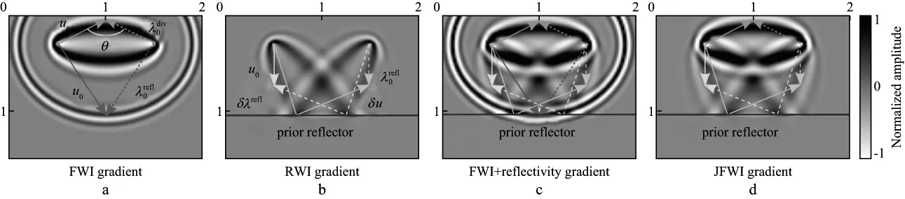
Figure 6 ).Note that the first Fresnel zone has a limited penetration in depth.(b) RWI gradient shows two wide first Fresnel zones centered on the two-way paths followed by the reflected wave between the reflector (behaving as a secondary source) and the source/receiver positions.(c) FWI gradient,with a prior reflectivity in the initial model,combines FWI (a) and RWI (b) gradients.Low-wavenumber and high-wavenumber information enter into the gradient,hence breaking down the scale-separation prerequisite.(d) JFWI gradient combines the first Fresnel zone generated by direct-wave residuals and RWI gradient.Compared with (c) the migration isochrone has been naturally removed and therefore honor the scale separation[75]
Kantorovich considers all the possible displacements allowing to fill the holes with the quantitiesqjfrom the sand pilespi.These displacements can be represented as matricesγwithNrows andMcolumns.An entryγijtells how much from the pilepishould be moved to fill in the holeqj.Mapping the ensemble of pilesponto the holesqrequires that the sum of the elements of theith row ofγijis equal topi,while the sum of the elements of thejth column ofγijis equal toqj.A matrix satisfying this assumption is called a “transport plan” and there is an infinity of possible transport plan.The OT prob-

Figure 7 Handling reflections:application of RWI and JFWI on the 2D synthetic Valhall case study.The true (e) VP and (f) IP model,and associated example of shot-gather (g).Inversion results using RWI for (a) VP and (b) IP.(c)-(d) same for the JFWI approach[75]

ENGQUIST & FROESE[93]illustrates the interesting behavior of the OT distance for FWI in a simple numerical experiment:measuring the OT distance between two timeshifted version of the same Ricker wavelet leads to a misfit function with a single minimum (no cycle-skipping) while standard least-squares norm presents two local minima aside the global minimum.
In MÉTIVIER et al[84-85],we extended this concept to a more general frame for FWI:first,our formulation was designed to handle problems without mass-conservation.For a seismic signal,mass is associated with the energy and there is no reason for the energy coming from the observed and calculated seismic traces to satisfy this assumption at the early stage of inversion.Second,our formulation considers seismic data as image or volume.Instead of using OT as a trace-by-trace measure,as proposed by ENGQUIST & FROESE[93],our formulation is working on the whole shot-gather panels.It is known from geophysicists for a long time that the manual identification of seismic events relies on their lateral coherency in trace-gather panels.Our formulation is,therefore,measuring the distance in the data-volume as an OT distance in a multi-dimensional space.Typically,for a time-domain FWI in 3D,that means that a 3D transport problem is considered to handle the time,inline and cross lines axis.This ability to account for the coherency of the seismic events not only in the time dimension but in the whole gather domain is a key feature of this optimal transport distance.
In order to develop a mathematical formulation of OT allowing for the previous criteria,we rely on solving a modified version of the Kantorovich problem.Indeed,handling different masses in the original Kantorovich is not possible,and the large dimensions of our trace gather panels measurement space prevent any linear programming technique from being efficient.Therefore,we rely on a dual formulation,proved to be equivalent than the first one[86,89],and defined as the Kantorovich-Rubinstein norm[91].In addition,to tackle large size measurement spaces,the problem has been reformulated as a non-smooth optimization problem,which can be solved efficiently through a proximal splitting algorithm named SDMM[94].
An example of OT-FWI performance is shown in Figure 8 on the 2D synthetic acoustic Marmousi model (Figure 8(a)).A fixed-spread surface acquisition with 128 sources each 125m and 168 receivers each 100m,at 50m depth is considered.A Ricker source function centered on 5Hz is used to generate the synthetic dataset,but the low-frequency content below 3Hz is suppressed with a high-pass filter in order to mimic realistic seismic data.Two initial models are considered:the first contains the main features of the exact model,only with smoother interfaces (Figure 8(b)).The second is a strongly smoothed version of the exact model with very weak lateral variations and underestimating the velocity in depth (Figure 8(c)).Starting from these two initial models,we compare the FWI results obtained using a least-squares distance and the OT distance we propose.The minimization is performed using thel-BFGS algorithm[95]implemented in the SEISCOPE optimization toolbox[96].The convergence to a correct estimation of the P-wave velocity model is obtained using both approaches (Figure 8(d) and(f)) when starting from a rather accurate initial model.However,when starting from a smoother model,only OT-FWI is able to converge toward meaningful result (Figure 8(g)).The poor initial model is responsible for cycle skipping and the difference-based misfit converges towards a local minimum (Figure 8(e)).This example illustrates the great potential of OT for FWI when starting models generate cycle-skipping.

Figure 8 Optimal-Transport based FWI on the Marmousi model case study.Exact model(a),initial model 1 (b),initial model 2 (c),results obtained with the least-squares distance starting from model 1 (d),from model 2 (e),results obtained with the OT approach starting from model 1 (f),from model 2 (g).
7 Conclusion and perspectives
FWI is now widely used in academia and industry for high-resolution quantitative imaging from seismic data.Despite its numerous successful applications at various scales,FWI is still facing significant issues for designing robust,efficient,systematic and automatic workflows.After presenting the basic mathematical ingredients of FWI as well as an analysis of equations and physics behind the FWI gradient,we reviewed three methodological approaches tackled recently in the SEISCOPE project:(1) algorithmic development for efficient building of the FWI gradient in 3D media including attenuation,based on the reverse propagation concept;(2) reformulation of the FWI to handle reflections for low-wavenumber update and coupling of the Reflection-oriented Waveform Inversion concept with transmission,leading to the Joint Full Waveform Inversion approach;(3) reformulation of the misfit function as an Optimal Transport measure,to mitigate the cycle-skipping problems.These developments show promising performances on synthetic studies and are currently investigated for real-data applications.
Acknowledgments
This study is funded by the SEISCOPE consortium (http:∥seiscope2.osug.fr) sponsored by CGG,CHEVRON,EXXON-MOBIL,JGI,SHELL,SINOPEC,STATOIL,TOTAL and WOODSIDE.The authors thank Stephane Operto for fruitful discussions.The authors appreciate BP Norge AS and Hess Norge AS for providing the Valhall synthetic models.This study is granted access to the HPC resources of the Froggy platform of the CIMENT infrastructure (https:∥ciment.ujf-grenoble.fr),which is supported by the Rhne-Alpes region (GRANT CPER07_13 CIRA),the OSUG@2020 labex (reference ANR10 LABX56) and the Equip@Meso project (reference ANR-10-EQPX-29-01) of the programme Investissements d’Avenir supervised by the Agence Nationale pour la Recherche,and the HPC resources of CINES/IDRIS under the allocation 046091 made by GENCI.
[1] LAILLY P.The seismic inverse problem as a sequence of before stack migrations[A].Conference on Inverse Scattering,1983:206-220
[2] TARANTOLA A.Inversion of seismic reflection data in the acoustic approximation[J].Geophysics,1984,49(8):1259-1266
[3] GAUTHIER O,VIRIEUX J,TARANTOLA A.Two-dimensional nonlinear inversion of seismic waveform:numerical results[J].Geophysics,1986,51(7):1387-1403
[4] TARANTOLA A.A strategy for non linear inversion of seismic reflection data[J].Geophysics,1986,51(10):1893-1903
[5] MORA P R.Nonlinear two-dimensional elastic inversion of multi-offset seismic data[J].Geophysics,1987,52(9):1211-1228
[6] MORA P R.Elastic wavefield inversion of reflection and transmission data[J].Geophysics,1988,53(6):750-759
[7] TARANTOLA A.Theoretical background for the inversion of seismic waveforms including elasticity and attenuation[J].Pure and Applied Geophysics,1988,128(1):365-399
[8] MORA P R.Inversion = migration+tomography[J].Geophysics,1989,54(12):1575-1586
[9] JANNANE M,BEYDOUN W,CRASE E,et al.Wavelengths of earth structures that can be resolved from seismic reflection data[J].Geophysics,1989,54(7):906-910
[10] CRASE E,PICA A,NOBLE M,et al.Robust elastic nonlinear waveform inversion:application to real data[J].Geophysics,1990,55(5):527-538
[11] PICA A,DIET J P,TARANTOLA A.Nonlinear inversion of seismic reflection data in laterally invariant medium[J].Geophysics,1990,55(3):284-292
[12] CRASE E,WIDEMAN C,NOBLE M,et al.Nonlinear elastic inversion of land seismic reflection data[J].Journal of Geophysical Research,1992,97(B4):4685-4705
[13] PRATT R G.Frequency-domain elastic modeling by finite differences:a tool for crosshole seismic imaging[J].Geophysics,1990,55(5):626-632
[14] PRATT R G,WORTHINGTON M H.Inverse theory applied to multi-source crosshole tomography,part Ⅰ:acoustic wave-equation method[J].Geophysical Prospecting,1990,38(3):287-310
[15] PRATT R G.Inverse theory applied to multi-source cross-hole tomography.part Ⅱ:elastic wave-equation method[J].Geophysical Prospecting,1990,38(3):311-330
[16] PRATT R G,SHIN C,HICKS G J.Gauss-Newton and full Newton methods in frequency-space seismic waveform inversion[J].Geophysical Journal International,1998,133(2):341-362
[17] PRATT R G.Seismic waveform inversion in the frequency domain,part Ⅰ:theory and verification in a physical scale model[J].Geophysics,1999,64(3):888-901
[18] PRATT R G,SHIPP R M.Seismic waveform inversion in the frequency domain,part Ⅱ:fault delineation in sediments using crosshole data[J].Geophysics,1999,64(3):902-914
[19] BUNKS C,SALEK F M,ZALESKI S,et al.Multiscale seismic waveform inversion[J].Geophysics,1995,60(5):1457-1473
[20] SIRGUE L,PRATT R G.Effcient waveform inversion and imaging:a strategy for selecting temporal frequencies[J].Geophysics,2004,69(1):231-248
[21] RAVAUT C,OPERTO S,IMPROTA L,et al.Multi-scale imaging of complex structures from multi-fold wide-aperture seismic data by frequency-domain full-wavefield inversions:application to a thrust belt[J].Geophysical Journal International,2004,159(3):1032-1056
[22] OPERTO S,VIRIEUX J,DESSA J X,et al.Crustal imaging from multifold ocean bottom seismometers data by frequency-domain full-waveform tomography:application to the eastern Nankai trough[J].Journal of Geophysical Research,2006,111(B09306):DOI:10.1029/2005JB003835
[23] BRENDERS A J,PRATT R G.Full waveform tomography for lithospheric imaging:results from a blind test in a realistic crustal model[J].Geophysical Journal International,2007,168(1):133-151
[24] BRENDERS A J,PRATT R G.Effcient waveform tomography for lithospheric imaging:implications for realistic 2D acquisition geometries and low frequency data[J].Geophysical Journal International,2007,168(1):152-170
[25] TAPE C,LIU Q,MAGGI A,et al.Seismic tomography of the southern California crust based on spectral-element and adjoint methods[J].Geophysical Journal International,2010,180(1):433-462
[26] SIRGUE L,BARKVED O I,DELLINGER J,et al.Full waveform inversion:the next leap forward in imaging at Valhall[J].First Break,2010,28(1728):65-70
[27] PETER D,KOMATITSCH D,LUO Y,et al.Forward and adjoint simulations of seismic wave propagation on fully unstructured hexahedral meshes[J].Geophysical Journal International,2011,186(2):721-739
[28] VIGH D,MOLDOVEANU N,JIAO K,et al.Ultralong-offset data acquisition can complement full-waveform inversion and lead to improved subsalt imaging[J].The Leading Edge,2013,32(9):1116-1122
[29] FICHTNER A,TRAMPERT J,CUPILLARD P,et al.Multiscale full waveform inversion[J].Geophysical Journal International,2013,194(1):534-556
[30] WARNERM,RATCLIFFE A,NANGOO T,et al.Anisotropic 3D full-waveform inversion[J].Geophysics,2013,78(2):R59-R80
[31] VIGH D,JIAO K,WATTS D,et al.Elastic full-waveform inversion application using multicomponent measurements of seismic data collection[J].Geophysics,2014,79(2):R63-R77
[32] STOPIN A,PLESSIX R E,AL ABRI S.Multiparameter waveform inversion of a large wide-azimuth low-frequency land data set in Oman[J].Geophysics,2010,75(3):WA69-WA77
[33] BORISOV D,SINGH S C.Three-dimensional elastic full waveform inversion in a marine environment using multicomponent ocean-bottom cables:a synthetic study[J].Geophysical Journal International,2015,201(3):1215-1234
[35] OPERTO S,MINIUSSI A,BROSSIER R,et al.Effcient 3-D frequency-domain mono-parameter full-waveform inversion of ocean-bottom cable data:application to Valhall in the visco-acoustic vertical transverse isotropic approximation[J].Geophysical Journal International,2015,202(2):1362-1391
[36] VIRIEUX J,OPERTO S.An overview of full waveform inversion in exploration geophysics[J].Geophysics,2009,74(6):WCC1-WCC26
[37] CHAVENT G.Nonlinear least squares for inverse problems[M].New York:Springer Dordrecht Heidelberg,2009:1-30
[38] TROMP J,TAPE C,LIU Q.Seismic tomography,adjoint methods,time reversal and banana-doughnut kernels[J].Geophysical Journal International,2005,160(1):195-216
[39] PLESSIX R E.A review of the adjoint-state method for computing the gradient of a functional with geophysical applications[J].Geophysical Journal International,2006,167(2):495-503
[40] NOCEDAL J,WRIGHT S J.Numerical optimization[M].Germany:Springer,2006:1-664
[41] WU R S,TOKSÖZ M N.Diffraction tomography and multisource holography applied to seismic imaging[J].Geophysics,1987,52(1):11-25
[42] SIRGUE L.Inversion de la forme d’onde dans le domaine fréquentiel de données sismiques grand offset[D].Canada:Queen’s University,2003
[43] SUN W,FU L Y.Two effective approaches to reduce data storage in reverse time migration[J].Computer & Geosciences,2013,56(56):69-75
[44] BOEHM C,HANZICH M,DELA P J,et al.Wavefield compression for adjoint methods in full-waveform inversion[J].Geophysics,2016,81(6):R385-R397
[45] PRABHAT,KOZIOL Q.High performance parallel I/O[M].London:Chapman and Hall/CRC,2014:1-434
[46] GRIEWANK A.Achieving logarithmic growth of temporal and spatial complexity in reverse automatic differentiation[J].Optimization Methods and Software,1992,1(1):35-54
[47] GRIEWANK A,WALTHER A.Algorithm 799:revolve:an implementation of checkpointing for the reverse or adjoint mode of computational differentiation[J].Acm Transactions on Mathematical Software,2000,26(1):19-45
[48] SYMES W W.Reverse time migration with optimal checkpointing[J].Geophysics,2007,72(5):SM213-SM221
[49] ANDERSON J E,TAN L,WANG D.Time reversal checkpointing methods for RTM and FWI[J].Geophysics,2012,77(4):S93-S103
[50] KOMATITSCH D,XIE Z,BOZDAG E,et al.An elastic sensitivity kernels with parsimonious storage for adjoint tomography and full waveform inversion[J].Geophysical Journal International,2016,206(3):1467-1478
[51] MITTET R.Implementation of the Kirchhoff integral for elastic waves in staggeredgrid modeling schemes[J].Geophysics,1994,59(12):1894-1901
[52] CLAPP R.Reverse time migration:saving the boundaries[R/OL].http://sepwww.stanford.edu/data/media/public/docs/sep136/bob4/paper.pdf
[53] DUSSAUD E,SYMES W W,WILLIAMSON P,et al.Computational strategies for reverse-time migration[J].Expanded Abstracts of 78thAnnual Internat SEG Mtg,2008:2267-2271
[54] BROSSIER R,PAJOT B,COMBE L,et al.Time and frequency-domain FWI implementations based on time solver:analysis of computational complexities[J].Expanded Abstracts of 76thAnnual Internat EAGE Mtg,2014:DOI:10.3997/2214-4609.20141139
[55] YANG P,GAO J,WANG B.RTM using effective boundary saving:a staggered grid GPU implementation[J].Computers & Geosciences,2014,68:64-72
[56] NGUYEN B D,MCMECHAN G A.Five ways to avoid storing source wavefield snapshots in 2D elastic prestack reverse time migration[J].Geophysics,2015,80(1):S1-S18
[57] RAKNES E B,WEIBULL W.Effcient 3D elastic full-waveform inversion using wavefield reconstruction methods[J].Geophysics,2016,81(2):R45-R55
[58] YANG P,BROSSIER R,VIRIEUX J,et al.Wavefield reconstruction from significantly decimated boundaries[J].Geophysics,2016,81(5):T197-T209
[59] VIRIEUX J.P-SV wave propagation in heterogeneous media:velocity-stress finite difference method[J].Geophysics,1986,51(4):889-901
[60] FORNBERG B.Generation of finite difference formulas on arbitrarily spaced grids[J].Mathematics of Computation,1988,51(184):699-706
[61] MOCZO P,KRISTEK J.On the rheological models used for time-domain methods of seismic wave propagation[J].Geophysical Research Letters,2005,32(1):L01306
[62] MOCZO P,ROBERTSSON J,EISNER L.The finite-difference time-domain method for modeling of seismic wave propagation[J].Advances in Geophysics,2007,48:421-516
[63] YANG P,BROSSIER R,MÉTIVIER L,et al.Wavefield reconstruction in attenuating media:a checkpointing-assisted reverse-forward simulation method[J].Geophysics,2016,81(6):R349-R362
[64] CLAERBOUT J.Imaging the earth’s interior[J].Dialogue & Universalism,1999,86(1):217
[65] CHAVENT G,CLÉMENT F,GóMEZ S.Automatic determination of velocities via migration-based traveltime waveform inversion:a synthetic data example[J].Expanded Abstracts of 64thAnnual Internat SEG Mtg,1994:1179-1182
[66] CHAVENT G.Duality methods for waveform inversion[R].1996:RR-2975,inria-00073723
[67] CLÉMENT F,CHAVENT G,GóMEZ S.Migration-based traveltime waveform inversion of 2-D simple structures:a synthetic example[J].Geophysics,2001,66(3):845-860
[68] XU S,WANG D,CHEN F,et al.Inversion on reflected seismic wave[J].Expanded Abstracts of 82ndAnnual Internat SEG Mtg,2012:1-7
[69] MA Y,HALE D.Wave-equation reflection traveltime inversion with dynamic warping and full waveform inversion[J].Geophysics,2013,78(6):R223-R233
[70] ALKHALIFAH T,WU Z.FWI and MVA the natural way[J].Expanded Abstracts of 76thEAGE Conference and Exhibition,2014:DOI:10.3997/2214-4609.20141091
[71] WU Z,ALKHALIFAH T.Full waveform inversion based on the optimized gradient and its spectral implementation[J].Expanded Abstracts of 76thAnnual Internat EAGE Mtg,2014:DOI:10.3997/2214-4609.20140706
[72] ALKHALIFAH T.Scattering angle based filtering of the waveform inversion gradients[J].Geophysical Journal International,2015,200(1):363-373
[73] BROSSIER R,OPERTO S,VIRIEUX J.Velocity model building from seismic reflection data by full waveform inversion[J].Geophysical Prospecting,2015,63(2):354-367
[74] WANG H,SINGH S,AUDEBERT F,et al.Inversion of seismic refraction and reflection data for building long-wavelengths velocity models[J].Geophysics,2015,80(2):R81-R93
[75] ZHOU W,BROSSIER R,OPERTO S,et al.Full waveform inversion of diving & reflected waves for velocity model building with impedance inversion based on scale separation[J].Geophysical Journal International,2015,202(3):1535-1554
[76] KOLB P,COLLINO F,LAILLY P.Prestack inversion of a 1-D medium[J].Proceedings of the IEEE,1986,74(3):498-508
[77] SHIPP R M,SINGH S C.Two-dimensional full wavefield inversion of wide-aperture marine seismic streamer data[J].Geophysical Journal International,2002,151(2):325-344
[78] WANG Y,RAO Y.Reflection seismic waveform tomography[J].Journal of Geophysical Research,2009,114(B3):63
[79] LUO Y,SCHUSTER G T.Wave-equation traveltime inversion[J].Geophysics,1991,56(5):645-653
[80] FICHTNER A,KENNETT B L N,IGEL H,et al.Theoretical background for continental-and global-scale full-waveform inversion in the time-frequency domain[J].Geophysical Journal International,2008,175(2):665-685
[82] LUO S,SAVA P.A deconvolution-based objective function for wave-equation inversion[J].Expanded Abstracts of 81stAnnual Internat SEG Mtg,2011:4424
[83] WARNER M,GUASCH L.Adaptative waveform inversion-FWI without cycle skipping-theory[J].Expanded Abstracts of 76thAnnual Internat EAGE Conference and Exhibition,2014:DOI:10.3997/2214-4609.20141092
[84] MÉTIVIER L,BROSSIER R,MÉRIGOT Q,et al.Measuring the misfit between seismograms using an optimal transport distance:application to full waveform inversion[J].Geophysical Journal International,2016,205(1):345-377
[85] MÉTIVIER L,BROSSIER R,MÉRIGOT Q,et al.An optimal transport approach for seismic tomography:application to 3D full waveform inversion,inverse problems,submitted[M].Camberley:Edward Elgar Publishing Ltd,2016:1-320
[86] VILLANI C.Topics in optimal transportation[J].Bulletin of the London Mathematical Society,2004,36(2):285-286
[87] VILLANI C.Optimal transport:old and new,Grundlehren der mathematischen Wissenschaften[M].Berlin:Springer,2008:1-976
[88] AMBROSIO L,GIGLI N,SAVARÉ G.Gradient ows:in metric spaces and in the space of probability measures[M].Berlin:Springer Science & Business Media,2008:DOI:10.1007/978-3-7643-8722-8
[89] SANTAMBROGIO F.Optimal transport for applied mathematicians:calculus of variations,PDEs,and modeling,progress in nonlinear differential equations and their applications[M/OL].http://vdisk.weibo.com/wap/s/d2XIcTV719VIb?sudaref=www.baidu.com
[90] FERRADANS S,PAPADAKIS N,PEYRÉ G,et al.Regularized discrete optimal transport[J].SIAM Journal on Imaging Sciences,2014,7(3):1853-1882
[91] LELLMANN J,LORENZ D,SCHONLIEB C,et al.Imaging with kantorovich-rubinstein discrepancy[J].SIAM Journal on Imaging Sciences,2014,7(4),2833-2859
[92] KANTOROVICH L.On the transfer of masses[J].Review of Politics,1942,51(4):551-580
[93] ENGQUIST B,FROESE B D.Application of the wasserstein metric to seismic signals[J].Communications in Mathematical Science,2014,12(5):979-988
[94] COMBETTES P L,PESQUET J-C.Proximal splitting methods in signal processing[J].Heinz H Bauschke,2010,49:185-212
[95] NOCEDAL J.Updating Quasi-Newton matrices with limited storage[J].Mathematics of Computation,1980,35(151):773-782
[96] MÉTIVIER L,BROSSIER R.The seiscope optimization toolbox:a large-scale nonlinear optimization library based on reverse communication[J].Geophysics,2016,81(2):F11-F25
(编辑:陈 杰)
2016-08-10;改回日期:2016-10-21。
Romain BROSSIER (1982—),Assistant professor at Université Grenoble Alpes Grenoble,France.Co-leader and permanent researcher of consortium SEISCOPE.His main research interests are high resolution quantitative imaging.
P631
A
1000-1441(2017)01-0003-17
10.3969/j.issn.1000-1441.2017.01.001
