Bayesian Saliency Detection for RGB-D Images

Songtao Wang Zhen Zhou Hanbing Qu Bin Li

1 Introduction

Saliency detection is the problem of identifying the points that attract the visual attention of human beings.Calletet al.introduced the concepts of overt and covert visual attention and the concepts of bottom-up and topdown processing[1].Visual attention selectively processes important visual information by fi ltering out less important information and is an important characteristic of the human visual system(HVS)for visual information processing.Visual attention is one of the most important mechanisms that are deployed in the HVS to cope with large amounts of visual information and reduce the complexity of scene analysis.Visual attention models have been successfully applied in many domains,including multimedia delivery,visual retargeting,quality assessment of images and videos,medical imaging,and 3D image applications[1].

Borjiet al.provided an excellent overview of the current state-of-the-art 2D visual attention modeling and included a taxonomy of models(cognitive,Bayesian,decision theoretic,information theoretical,graphical,spectral analysis,pattern classi fi cation,and more)[2].Many saliency measures have emerged that simulate the HVS,which tends to fi nd the most informative regions in 2D scenes[3]−[10].However,most saliency models disregard the fact that the HVS operates in 3D environments and these models can thus investigate only from 2D images.Eye fi xation data are captured while looking at 2D scenes,but depth cues provide additional important information about content in the visual fi eld and therefore can also be considered relevant features for saliency detection.The stereoscopic content carries important additional binocular cues for enhancing human depth perception[11],[12].Today,with the development of 3D display technologies and devices,there are various emerging applications for 3D multimedia,such as 3D video retargeting[13],3D video quality assessment[14],[15],3D ultrasound images processing[16],[17]and so forth.Overall,the emerging demand for visual attentionbased applications for 3D multimedia has increased the need for computational saliency detection models for 3D multimedia content.In contrast to saliency detection for 2D images,the depth factor must be considered when performing saliency detection for RGB-D images.Therefore,two important challenges when designing 3D saliency models are how to estimate the saliency from depth cues and how to combine the saliency from depth features with those of other 2D low-level features.

In this paper,we propose a new computational saliency detection model for RGB-D images that considers both color-and depth-based contrast features within a Bayesian framework.The main contributions of our approach consist of two aspects:1)to estimate saliency from depth cues,we propose the creation of depth feature maps based on superpixel contrast computation with spatial priors and model the depth saliency map by approximating the density of depth-based contrast features using a Gaussian distribution,and 2)by assuming that color-based and depth-based features are conditionally independent given the classes,the discriminative mixed-membership naive Bayes(DMNB)model is used to calculate the fi nal saliency map by applying Bayes’theorem.

The remainder of this paper is organized as follows.Section 2 introduces the related work in the literature.In Section 3,the proposed model is described in detail.Section 4 provides the experimental results on eye tracking databases.The fi nal section concludes the paper.

2 Related Work

As introduced in Section 1,many computational models of visual attention have been proposed for various 2D multimedia processing applications.However,compared with the set of 2D visual attention models,only a few computational models of 3D visual attention have been proposed[18]−[36]. These models all contain a stage in which 2D saliency features are extracted and used to compute 2D saliency maps.However,depending on the way in which they use depth information in terms of the development of computational models,these models can be classi fi ed into three different categories:

1)Depth-weighting Models:This type of model adopts depth information to weight a 2D saliency map to calculate the fi nal saliency map for RGB-D images with feature map fusion[18]−[21].Fanget al.proposed a novel 3D saliency detection framework based on color,luminance,texture and depth contrast features,which designed a new fusion method to combine the feature maps to obtain the fi nal saliency map for RGB-D images[18].Ciptadiet al.proposed a novel computational model of visual saliency that incorporates depth information and demonstrated the method by explicitly constructing 3D layout and shape features from depth measurements[19].In[20],color contrast features and depth contrast features are calculated to construct an effective multi-feature fusion to generate saliency maps,and multi-scale enhancement is performed on the saliency map to further improve the detection precision focused on the 3D salient object detection.The models in this category combine 2D features with a depth feature to calculate the fi nal saliency map,but they do not include the depth saliency map in their computation processes.Apart from detecting the salient areas by using 2D visual features,these models share a common step in which depth information is used as a weighting factor for the 2D saliency.

2)Depth-pooling Models:This type of model combines depth saliency maps and traditional 2D saliency maps to simply obtain saliency maps for RGB-D images[11],[12],[22]−[32].Ouerhaniet al.aimed at extension of the visual attention model to the depth component of the scene.They attempted to integrate depth into the computational model built around conspicuity and saliency maps[23].Desinghet al.investigated the role of depth in saliency detection in the presence of competing saliencies due to appearance,depth-induced blur and centre-bias and proposed a 3D-saliency formulation in conjunction with 2D saliency models through non-linear regression using a support vector machine(SVM)to improve saliency[12].Xueet al.proposed an effective visual object saliency detection model via RGB and depth cues mutual guided manifold ranking and obtained the fi nal result by fusing RGB and depth saliency maps[24].Renet al.presented a two-stage 3D salient object detection framework,which fi rst integrates the contrast region with the background,depth and orientation priors to achieve a saliency map and then reconstructs the saliency map globally[25].Songet al.proposed an effective saliency model to detect salient regions in RGBD images through a location prior of salient objects integrated with color saliency and depth saliency to obtain the regional saliency map[26].Guoet al.proposed a saliency fusion and propagation strategy-based salient object detection method for RGB-D images,in which the saliency maps based on color cues,location cues and depth cues are independently fused to provide high precision detection results,and saliency propagation is utilized to improve the completeness of the salient objects[27].Fanet al.proposed an effective saliency model that combines region-level saliency maps generated using depth,color and spatial information to detect salient regions in RGB-D images[28].Penget al.proved a simple fusion framework that combines existing RGB-produced saliency with new depth-induced saliency:the former one is estimated from existing RGB models,while the latter one is based on the multi-contextual contrast model[29].In[30],stereo saliency based on disparity contrast analysis and domain knowledge from stereoscopic photography was computed.Furthermore,Juet al.proposed a novel saliency method that worked on depth images based on anisotropic centre-surround difference[31].Wanget al.proposed two different ways of integrating depth information in the modeling of 3D visual attention,where the measures of depth saliency are derived from the eye movement data obtained from an eye tracking experiment using synthetic stimuli[32].Langet al.analyzed the major discrepancies between 2D and 3D human fi xation data of the same scenes,which are further abstracted and modelled as novel depth priors with a mixture of Gaussians[11].To investigate whether the depth saliency is helpful for determining 3D saliency,some existing 2D saliency detection method are combined[12],[22],[31].Iatsunet al.proposed a 3D saliency model relying on 2D saliency features jointly with depth obtained from monocular cues,in which 3D perception is signi fi cantly based on monocular cues[22].The models in this category rely on the existence of “depth saliency maps”.Depth features are extracted from the depth map to create additional feature maps,which are then used to generate the depth saliency maps(DSM).These depth saliency maps are fi nally combined with 2D saliency maps using a saliency map pooling strategy to obtain a fi nal 3D saliency map.

3)Learning-based Models:Instead of using a depth saliency map directly,this type of model uses machine learning techniques to build a 3D saliency detection model for RGB-D images based on extracted 2D features and depth features[31]−[36].Iatsunet al.proposed a visual attention model for 3D video using a machine learning approach.They used arti fi cial neural networks to de fi ne adaptive weights for the fusion strategy based on eye tracking data[33].Inspired by the recent success of machine learning techniques in building 2D saliency detection models,Fanget al.proposed a learning-based model for RGBD images using linear SVM[34].Zhuet al.proposed a learning-based approach for extracting saliency from RGBD images,in which discriminative features can be automatically selected by learning several decision trees based on the ground truth,and those features are further utilized to search the saliency regions via the predictions of the trees[35].Bertasiuset al.developed an EgoObject representation,which encodes these characteristics by incorporating shape,location,size and depth features from an egocentric RGB-D image,and trained a random forest regressor to predict the saliency of a region using ground truth salient object[36].

From the above description,the key to 3D saliency detection models is determining how to integrate the depth cues with traditional 2D low-level features.In this paper,we propose a learning-based 3D saliency detection model with a Bayesian framework that considers both color-and depth-based contrast features.Instead of simply combining a depth map with 2D saliency maps as in previous studies,we propose a computational saliency detection model for RGB-D images based on the DMNB model[37].Experimental results from a public eye tracking database demonstrate the improved performance of the proposed model over other strategies.

3 The Proposed Approach

In this section,we introduce a method that integrates the color saliency probability with the depth saliency probability computed from Gaussian distributions based on multiscale superpixel contrast features and yields a prediction of the fi nal 3D saliency map using the DMNB model within a Bayesian framework.First,the input RGB-D images are represented by superpixels using multi-scale segmentation.Then,we compute the color and depth map using the weighted summation and normalization of the colorand depth-based contrast features,respectively,at different scales.Second,the probability distributions of both the color and depth saliency are modelled using the Gaussian distribution based on the color and depth feature maps,respectively.The parameters of the Gaussian distribution can be estimated in the DMNB model using a variational inference-based expectation maximization(EM)algorithm.The general architecture of the proposed framework is presented in Fig.1.

3.1 Feature Extraction Using Multi-scale Superpixels

We introduce a color-based contrast feature and a depthbased contrast feature to capture the contrast information of salient regions with spatial priors based on multi-scale superpixels,which are generated at various grid interval parametersS,similar to simple linear iterative clustering(SLIC)[38].We further impose a spatial prior term on each of the contrast measures holistically,which constrains the pixels that were rendered as salient to be compact as well as centred in the image domain.This spatial prior can also be generalized to consider the spatial distribution of different saliency cues such as the centre prior and background prior[10],[29].We also observe that the background often presents local or global appearance connectivity with each of four image boundaries.These two features complement each other in detecting 3D saliency cues from different perspectives and,when combined,yield the fi nal 3D saliency value.

1)RGB-D Images Multi-scale Superpixel Segmentation:For an RGB-D image pair,superpixels are segmented according to both color and depth cues.We notice that when applying the SLIC algorithm directly to the RGB image and depth map,the segmentation result is unsatisfactory due to the lack of a mutual context relationship.We rede fi ne the distance measurement incorporating depth as shown in(1):

We obtain more accurate segmentation results as shown in Fig.2 by considering the color and depth cues simultaneously.The boundary between the foreground and the background is segmented more accurately.

Algorithm 1.Superpixel segmentation of the RGB-D images

Input:m,S,ωdandIterNum.

Initialization:Initialize clustersCi=[li,ai,bi,di,xi,yi]Tby sampling pixels at regular grid stepsSby computing the averagelabdxyvector,where[li,ai,bi]is theL,a,bvalues of the CIELAB color space and[xi,yi]is the pixel coordinates ofith grid in the RGB-D image pair.

Set labell(p)=−1 and distanced(p)=∞for each pixelp.

Output:d(p).

1:Perturb cluster centres in a 3×3 neighbourhood to the lowest gradient position in the RGB image.

2:forIterNumdo

3:foreach cluster centreCido

4:Assign the best matching pixels from a 2S×2Ssquare neighbourhood around the cluster centre according to the distance measureDsin(1).

for each pixel p in a 2S×2Sregion aroundCido

Compute the distanceDsbetweenCiandlabdxyp

ifDs＜d(p)then

Setd(p)=Ds

Setl(p)=i

end if

end for

5:end for

6:Computer new cluster centres.After all the pixels are associated with the nearest cluster center,a new center is computed as the averagelabdxyvector of all the pixels belonging to the cluster.

7:end for

8:Enforce connectivity.

2)Color-based Contrast feature:An input image is oversegmented atLscales,and the color feature map is formulated as

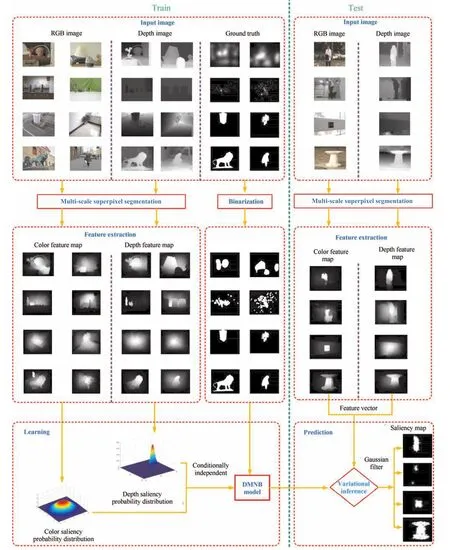
Fig.1. The fl owchart of the proposed model.The framework of our model consists of two stages:the training stage shown in the left part of the fi gure and the testing stage shown in the right part of the fi gure.In this work,we perform experiments based on the EyMIR dataset in[32],NUS dataset in[11],NLPR dataset in[29]and NJU-DS400 dataset in[31].

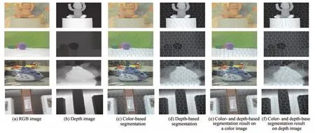
Fig.2.Visual samples for superpixel segmentation of RGB-D images with S=40.Rows 1−4:comparative results on the EyMIR dataset,NUS dataset,NLPR dataset and NJU-DS400 dataset,respectively.

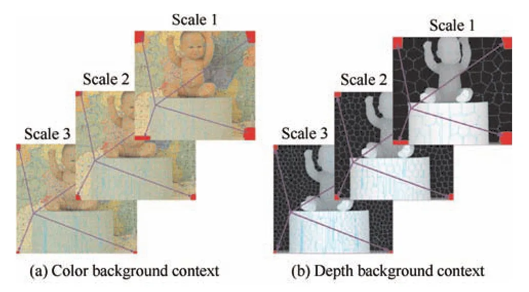
Fig.3. Visual illustration for the saliency measure based on manifold ranking,where patches from corners of images marked as red is de fi ned as pseudo-background.

With multi-scale fusion,the color feature map is constructed by weighted sum mation of,where the weights are determined by.The fi nal pixelwise color feature map is obtained by assigning the feature value of each superpixel to every pixel belonging to it,as shown in the fi rst row of Fig.4.

3)Depth-based Contrast Feature:Similar to the construction of the color feature maps,we formulate the depth feature maps based on multi-scale superpixels in the depth maps:

4)Bayesian Framework for Saliency Detection:Let the binary random variabledenote whether a point belongs to a salient class.Given the observed color-based contrast featureand the depth-based contrast featureof that point,we formulate the saliency detection as a Bayesian inference problem to estimate the posterior probability at each pixel of the RGB-D image:

In this paper,the class-conditional mutual information(CMI)is used as a measure of dependence between two featuresand,which can be de fi ned as,is the class-conditional entropy of,de fi ned as.Mutual information is zero whenandare mutually independent given classand,increases with increasing level of dependence,reaching the maximum when one feature is a deterministic function of the other.Indeed,the independence assumption becomes more accurate with decreasing entropy which yields an asymptotically optimal performance of the naive Bayes classi fi er[39].

We employ a CMI thresholdτto discover feature dependencies,as shown in Fig.5.For CMI between the colorbased contrast feature and depth-based contrast feature less thanτ,we assume thatandare conditionally independent given the classes,that is,. This entails the assumption that the distribution of the color-based contrast features does not change with the depth-based contrast features.Thus,the pixel-wise saliency of the likelihood is given by.

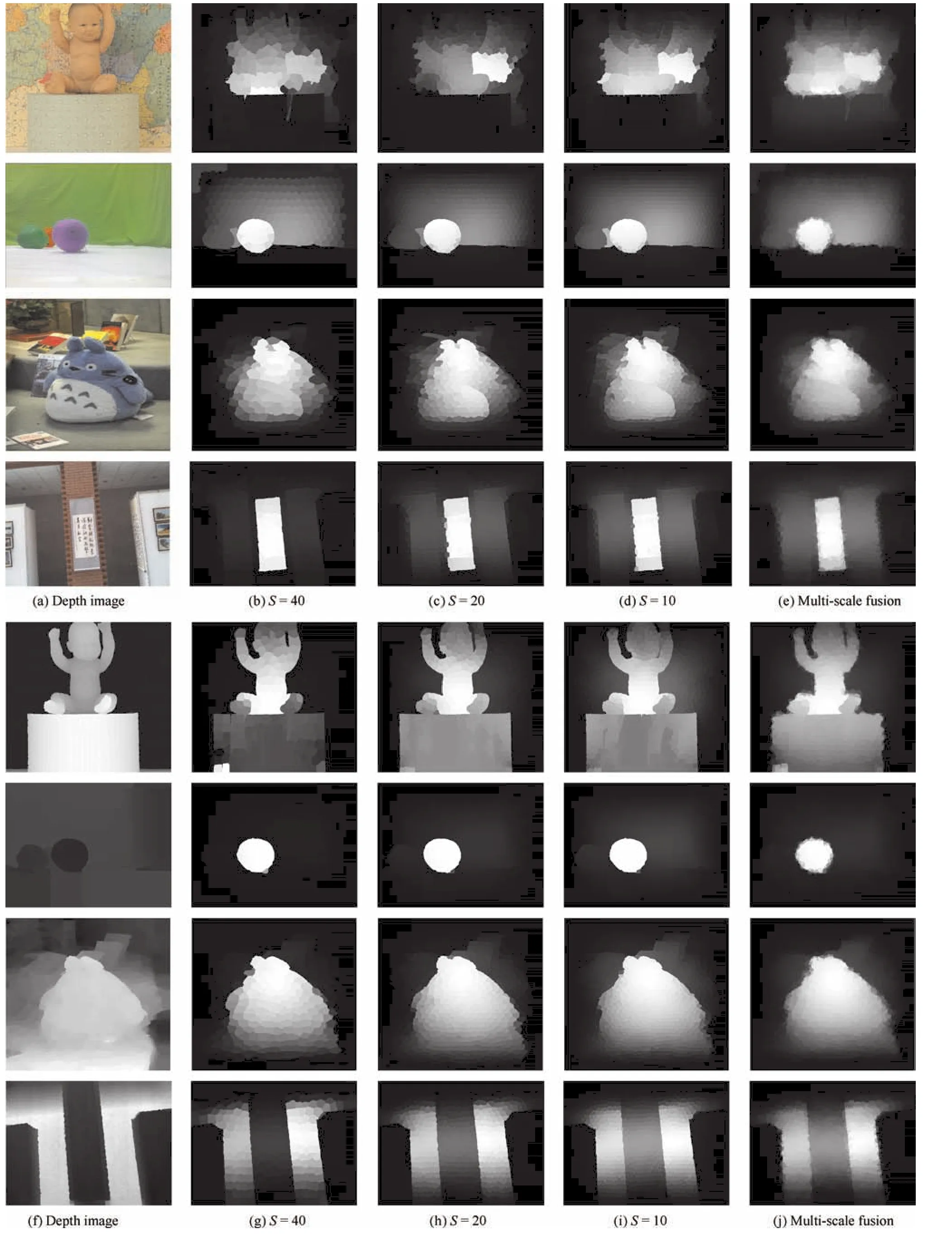
Fig.4. Visual samples of different color and depth feature maps.Rows 1−4:color feature maps of the EyMIR dataset,NUS dataset,NLPR dataset and NJU-DS400 dataset,respectively.Rows 5−8:depth feature maps of the EyMIR dataset,NUS dataset,NLPR dataset and NJU-DS400 dataset,respectively.

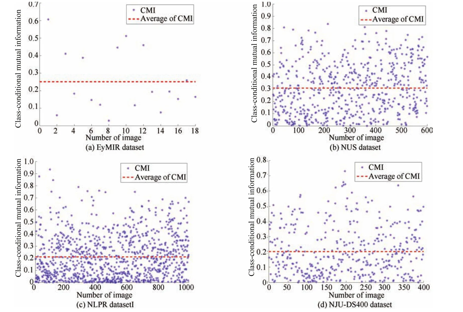
Fig.5. Visual results for class-conditional mutual information between color-based contrast features and depth-based contrast features on four RGB-D image datasets.

3.2 DMNB Model for Saliency Estimation

By assuming that color and depth features are conditional independent given class,the DMNB model is adopted to calculate the fi nal saliency map from the depth saliency probability and color saliency probability by applying Bayess theorem.DMNB could be considered as a generalization of NB classi fi er extend in the following aspects:First,NB shares a component among all features,but DMNB has a separate component for each feature and maintains a Dirichlet-multinomial prior on all possible combination of component assignments.Second,NB uses the shared component as a class indicator,whereas DMNB uses the mixed membership over separate components as inputs to a logistic regression model which fi nally generates the class label.In this paper,the DMNB model has Gaussian distribution for each color and depth feature and is applicable to predict fi nal saliency map.

Given the graphical model of DMNB for saliency detection shown in Fig.6,the generative process for{x1:N,y}following the DMNB model can be described as Algorithm 2,wherep(·|α)is a Dirichlet distribution parameterized byα,θis sampled from ap(θ|α)distribution,p(·|θ)is a multinomial distribution parameterized byθ,,is an exponential family distribution for featuregiven the hidden classparameterized by Ωj,is a multi-class logistic regression forandis the label that indicates whether the pixel is salient or not.

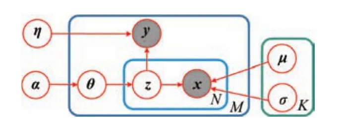
Fig.6.Graphical models of DMNB for saliency estimation. y and x are the corresponding observed states,and z is the hidden variable.

Algorithm 2. Generative process for saliency detection following the DMNB model

Due to the latent variables,the computation of the likelihood in(7)is intractable.In this paper,we use a variational inference method,which alternates between obtaining a tractable lower bound to the true log-likelihood and choosing the model parameters to maximize the lower bound.

For each feature value,to obtain a tractable lower bound to logp,we introduce a variational distributionas an approximation of the true posterior distributionover the latent variable.By a direct application of Jensen’s inequality[37],the lower bound to logis given by

whereq(θ,γ)is aK-dimensional Dirichlet distribution forθ,is Discrete distribution for.We useLto denote the lower bound:

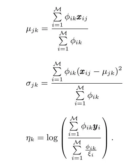
The variational parameters(γ∗,φ∗,ξ∗)from the inference step provide the optimal lower bound for the loglikelihood of,and maximizing the aggregate lower boundover all of the data with respect toα, Ω andη,respectively,yields the estimated parameters.

Variational parameters(γ∗,φ∗,ξ∗)from the inference step gives the optimal lower bound to the log-likelihood of,and maximizing the aggregate lower boundover all data points with respect toα, Ω andη,respectively,yields the estimated parameters.As forµ,σandη,we have

Based on the variational inference and parameter estimation updates,it is straightforward to construct a variant EM algorithm to estimate(α, Ω,andη).Starting with an initial guess(α0,Ω0,andη0),the variational EM algorithm alternates between two steps,as Algorithm 3.

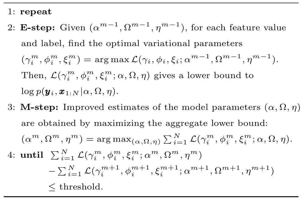
Algorithm 3.Variational EM algorithm for DMNB

After obtaining the DMNB model parameters from the EM algorithm,we can useηto perform saliency prediction.Given the feature,we have

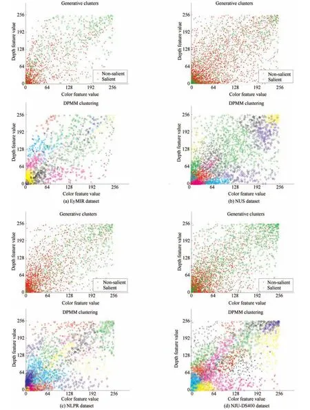
Fig.7.Visual result for the number of components K in the DMNB model:generative clusters vs DPMM clustering.Row 1:generative clusters for four RGB-D image datasets,where green and red denote distribution of salient and non-salient features,respectively.Row 2:DPMM clustering for four RGB-D image datasets,where the number of colors and shapes of the points denote the number of components K.The appropriate number of mixture components to use in DMNB model for saliency estimation is generally unknown,and DPMM provides an attractive alternative to current method.We fi nd K=26,34,28,and 32 using DPMM on the EyMIR dataset,NUS dataset,NLPR dataset and NJU-DS400 dataset,respectively.

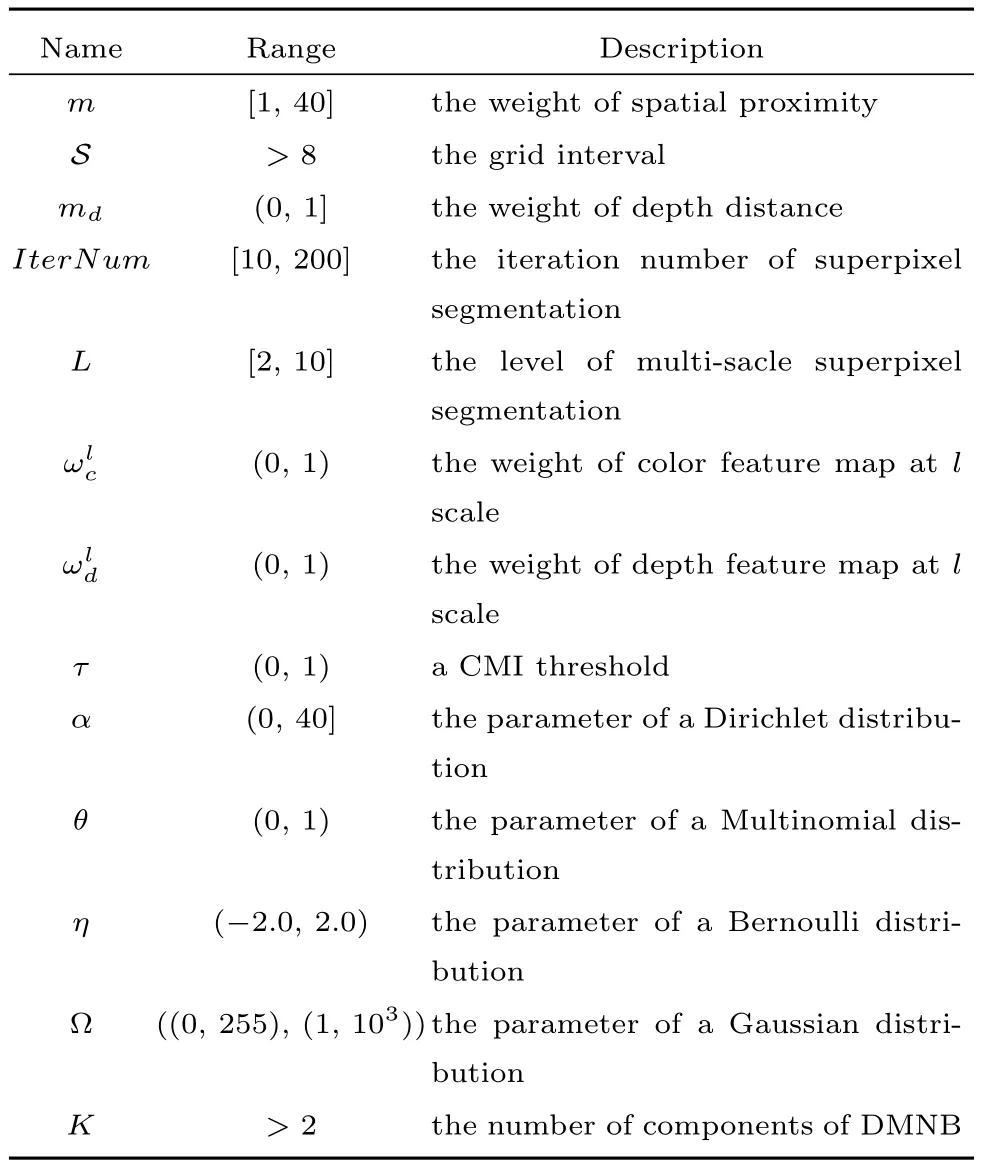
TABLE ISUMMARY OF PARAMETERS

4 Experimental Evaluation

4.1 Experimental Setup

1)Dataset:In this section,we conduct some experiments to demonstrate the performance of our method.We use four databases to evaluate the performance of the proposed model,as shown in Table II.We distinguish between two cases.The fi rst case includes images that show a single salient object over an uninteresting background.For such images,we expect that only the object’s pixels will be identi fi ed as salient.The fi rst databases were presented in the NLPR dataset1http://sites.google.com/site/rgbdsaliencyand NJU-DS400 dataset2http://mcg.nju.edu.cn/en/resource.html.The NLPR dataset includes 1000 images of diverse scenes in real 3D environments,where the ground-truth was obtained by requiring fi ve participants to select regions where objects are presented,i.e.,the salient regions were marked by hand.The NJU-DS400 dataset includes 400 images of different scenes,where the ground-truth was obtained by four volunteers labelling the salient object masks.The second case includes images of complex scenes.The EyMIR dataset3http://www.irccyn.ecnantes.fr/spip.php?article1102&lang=enand NUS dataset4https://sites.google.com/site/vantam/nus3d-saliency-datasetare somewhat different.In these datasets,the images were presented to human observers for several seconds each,and eye tracking data were collected and averaged.In the NUS dataset,Langet al.collected a large human eye fi xation database from a pool of 600 2D-vs-3D image pairs viewed by 80 subjects,where the depth information is directly provided by the Kinect camera and the eye tracking data are captured in both 2D and 3D free-viewing experiments.In the EyMIR dataset,10 images from the database were selected from the Middlebury 2005/2006 image dataset,and the rest of the database consisted of the set of images from the IVC 3D image dataset,which contains two outdoor scenes and six indoor scenes.To create the ground-truth map,observers viewed the stereoscopic stimuli through a pair of passive polarized glasses at a distance for 15 seconds.

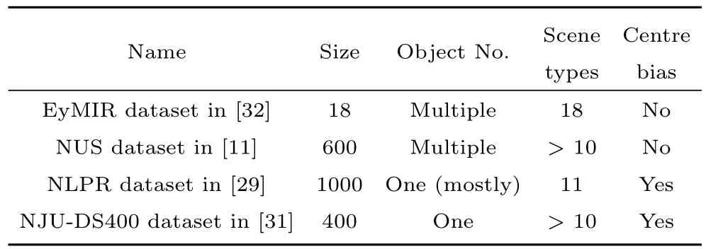
TABLE II COMPARISON OF THE BENCHMARK AND EXISTING 3D SALIENCY DETECTION DATASETS

2)Evaluation Metrics:To date,there are no speci fi c and standardized measures for computing the similarity between the fi xation density maps and saliency maps created using computational models in 3D situations.Nevertheless,there is a range of different measures that are widely used to perform comparisons of saliency maps for 2D content.We introduce two types of measures to evaluate algorithm performance on the benchmark.The fi rst one is the gold standard:F-measure.The F-measure is the overall performance measurement computed by the weighted harmonic of precision and recall:

where we setβ2=0.3 to emphasize the precision[5].Precision corresponds to the percentage of salient pixels correctly assigned to all the pixels of extracted regions,and Recall is the fraction of detected salient pixels belonging to the salient object in the ground truth.The F-measure is computed with an adaptive saliency threshold that is de fi ned as twice the mean saliency of the image[5].The adaptive threshold is de fi ned as

whereWandHdenote the width and height of an image,respectively.

The second is the receiver operating characteristic(ROC)curve and the area under the ROC curve(AUC).By thresholding over the saliency maps and plotting true positive rate vs.false positive rate,an ROC curve is acquired.The AUC score is calculated as the area underneath the ROC.

3)Parameter Setting:To evaluate the quality of the proposed approach,we divided the datasets into two subsets according to their CMI values,and we held out 90%of the data whose CMI values are less thanτfor training purpose and tested on the remaining 10%.For each image,we chose positively labelled samples randomly from the top 40%of salient locations in the human fi xation maps and negatively labelled samples from the bottom 30%of salient locations to construct training sets based on the NUS dataset and the EyMIR dataset.The ground truth is binarized by the adaptive threshold in(16).We set theIterNum=10,m=20 andωd=1.0 in Algorithm 1.We set theL=3,ωcl=0.2,0.3,0.5,ωdl=0.3,0.3,0.4 andσ2=0.1 in(2),(4)and(5),respectively.As shown in Fig.5,we compute the CMI for all of the RGB-D images,and the parameterτis set to 0.35,which is a heuristically determined value.We initialize the model parameters using all data points and their labels in the training set in Algorithm 2.In particular,we use the mean and standard deviation of the data points in each class to initialize Ω andDc/Dto initializeαi,whereDcis the number of data points in classcandDis the total number of data points.For theηin the DMNB model,we run a cross validation by holding out 10%of the training data as the validation set and use the parameters generating the best results on the validation set.We fi nd the initial number of componentsKusing the DPMM based on 90%of the training dataset.

Our algorithm is implemented in MATLAB v7.12 and tested on a Intel Core(TM)2 Quad CPU 2.33GHz with 4GB RAM.A simple computational comparison is shown in Table III in terms of EyMIR,NUS,NLPR and NJUDS400 datasets.It should be noted that there are lots of works left for computational optimization,including prior parameters optimization,algorithm optimization for variable inference during the prediction process.

TABLE III COMPARISON OF THE AVERAGE RUNNING TIME(SECONDS PER RGB-D IMAGE PAIR)ON THE EYMIR,NUS,NLPR AND NJU-DS400 DATASETS(S)

4)The Effect of the Parameters:In particular,we performed the experiments while varyingSfrom Algorithm 1 andKfrom Algorithm 2.Fig.8 shows typical results when varyingSfrom Algorithm 1.Fig.8 illustrates the AUC obtained from the different numbers of superpixels.If only one scale is used,the results are inferior.This justi fi es our multi-scale approach.

The parameterKis the number of components in the proposed algorithm,and we set a larger number of components than the number of classes in this paper.Interesting,a largerKhelps to discover the components not speci fi ed in labels and increase classi fi cation accuracy.The appropriate number of mixture components to use in DMNB model for saliency estimation is generally unknown,and DPMM provides an attractive alternative to current method.In practice,we fi nd the initial number of componentsKusing the DPMM based on 90%of the training set,then we run a cross validation with a range ofKby holding out 10%of the training data as the validation.We use 10-fold cross-validation with the parameterKfor DMNB models.In a 10-fold cross-validation,we divide the dataset evenly into 10 parts,one of which is picked as the validation set,and the remaining 9 parts are used as the training set.The process is repeated 10 times,with each part used once as the validation set.We use perplexity as the measurement for comparison.The generative models are capable of assigning a log-likelihood logto each observed data point.Based on the log-likelihood scores,we compute the perplexity of the entire dataset as,wherenis the number of data points.The perplexity is a monotonically decreasing function of the log-likelihood,implying that lower perplexity is better(especially on the test set)since the model can explain the data better.We calculate the perplexity for results on the validation set and training set respectively.

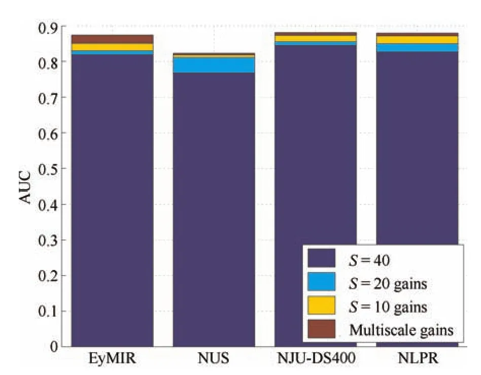
Fig.8. The effects of the number of scales S on the EyMIR,NUS,NLPR and NJU-DS400 datasets.A single scale produces inferior results.

The parameterKin Algorithm 2 is set according to the training set based on DPMM,as shown in Fig.7.Given a range of values for the number of componentsK,the overall results on training and test sets are presented as perplexity in Fig.9.For a generative model,a larger number of parameters may yield a better performance on the training set,such as a lower perplexity or a higher accuracy,since the model could be as complicated as necessary to fi t the training data perfectly well.However,such complicated models typically lose the ability for generalization and lead to over- fi tting on the test set.If the over- fi tting does occur to DMNB,it will lead to a bad performance on the test set.Thus the results on test sets are more interesting and crucial.Finally,for all the experiments described below,the parameterKwas fi xed at 32—no user fi ne-tuning was done.

We are also interested in the contributions of different features in our model.The ROC curves of saliency estimation from different features are shown in Fig.10.This may be why the color and depth saliency maps show comparable performances,whereas their combination produces a much better result.

4.2 Qualitative Experiment

During the experiments,we compare our algorithm with fi ve state-of-the-art saliency detection methods,among which three are developed for RGB-D images and two for traditional 2D image analysis.One RGB-D method performs saliency detection at low-level,mid-level,and highlevel stages and is therefore referred to as LMH[29].One RGB-D method is based on anisotropic centre-surround difference and is therefore denoted ACSD[31].The other RGB-D method exploits global priors,which include the background,depth,and orientation priors to achieve a saliency map and is therefore denoted GP[25].The two 2D methods are Hemami’s frequency-tuned method[15],which is denoted FT,and the approach from the graphbased manifold ranking[10],which is denoted GMR.For the two 2D saliency approaches,we also add and multiple their results with the DSM produced by our proposed depth feature map;these results are denoted FT+DSM,FT×DSM,GMR+DSM and GMR×DSM.All of the results are produced using public codes that are offered by the authors of the previously mentioned literature reports.

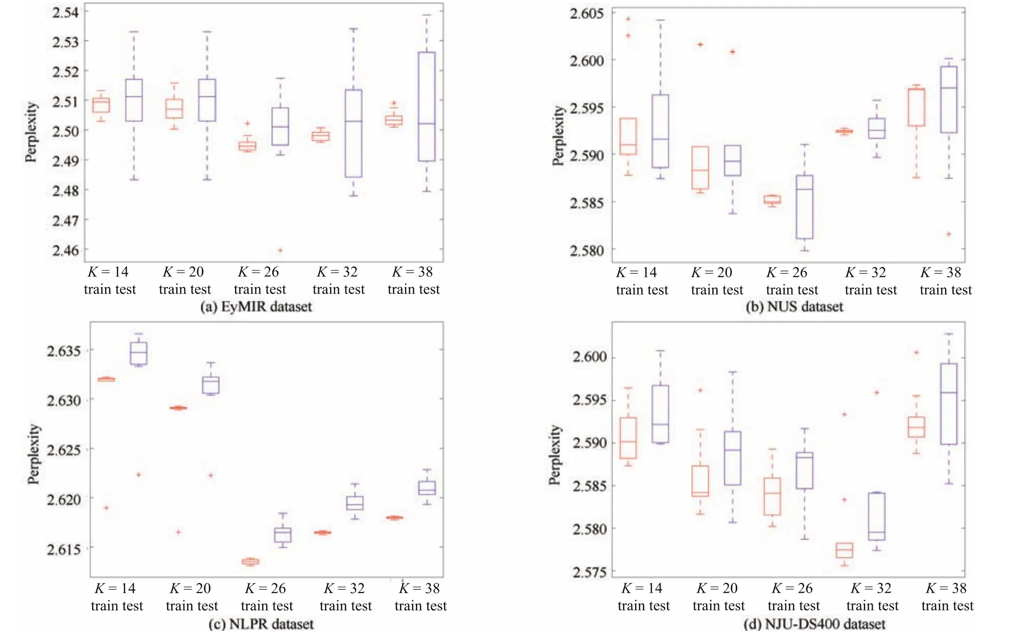
Fig.9. The perplexity for different K components in the DMNB model in terms of the four datasets.We use 10-fold cross-validation with the parameter K for DMNB models.The K found using DPMM was adjusted over a wide range in a 10-fold cross-validation.

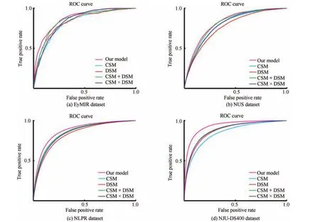
Fig.10. The ROC curves of different feature map and their linear fusions.+indicates a linear combination strategy,and × indicates a weighting method based on multiplication.

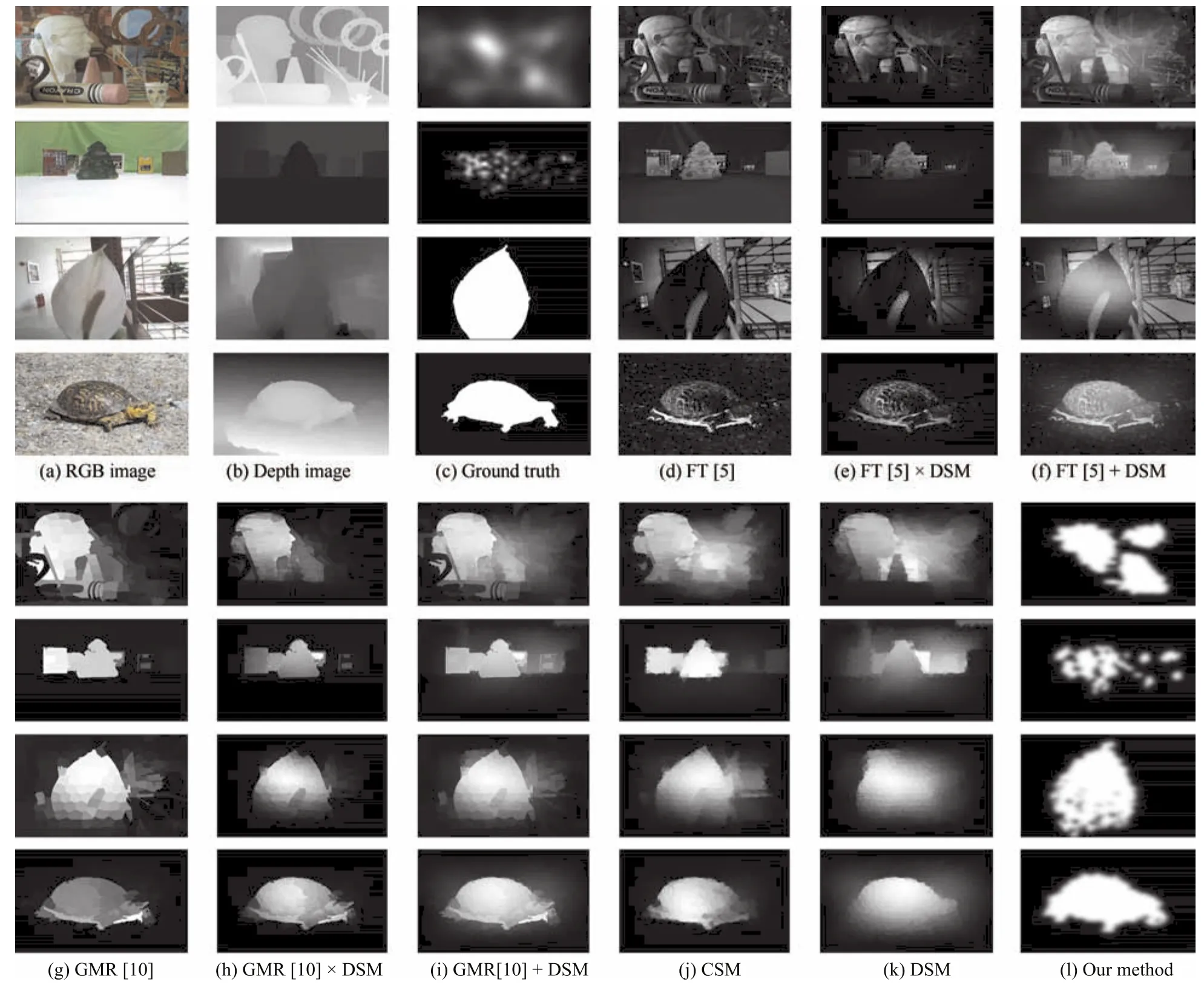
Fig.11.Visual comparison of the saliency estimations of the different 2D methods with DSM.+indicates a linear combination strategy,and×indicates a weighting method based on multiplication.DSM means depth saliency map,which is produced by our proposed depth feature map.CSM means color saliency map,which is produced by our proposed color feature map.

Fig.11 compares our results with FT[5],FT+DSM,FT×DSM,GMR[10],GMR+DSM and GMR×DSM.As shown in Fig.11,FT detects many uninteresting background pixels as salient because it does not consider any global features.The experiments show that both FT+DSM and FT×DSM are highly improved when incorporated with the DSM.GMR fails to detect many pixels on the prominent objects because it does not de fi ne the pseudo-background accurately.Although the simple late fusion strategy achieves improvements,it still suffers from inconsistency in the homogeneous foreground regions and lacks precision around object boundaries,which may be ascribed to treating the appearance and depth correspondence cues in an independent manner.Our approach consistently detects the pixels on the dominant objects within Bayesian framework with higher accuracy to resolve the issue.

The comparison of the ACSD[31],LMH[29]and GP[25]RGB-D approaches is presented in Figs.12−15.ACSD works on depth images on the assumption that salient objects tend to stand out from the surrounding background,which takes relative depth into consideration.In Fig.13,ACSD generates unsatisfying results without color cues.LMH uses a simple fusion framework that takes advantage of both depth and appearance cues from the low-,mid-,and high-levels.In[29],the background is nicely excluded;however,many pixels on the salient object are not detected as salient,as shown in Fig.14.Renet al.proposed two priors,which are the normalized depth prior and the globalcontext surface orientation prior[25].Because their approach uses the two priors,it has problems when such priors are invalid,as shown in Fig.12.We can see that the proposed method can accurately locate the salient objects and produce nearly equal saliency values for the pixels within the target objects.

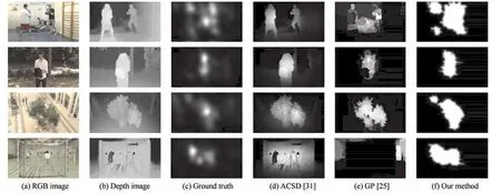
Fig.12. Visual comparison of saliency estimations of different 3D methods based on the EyMIR dataset.

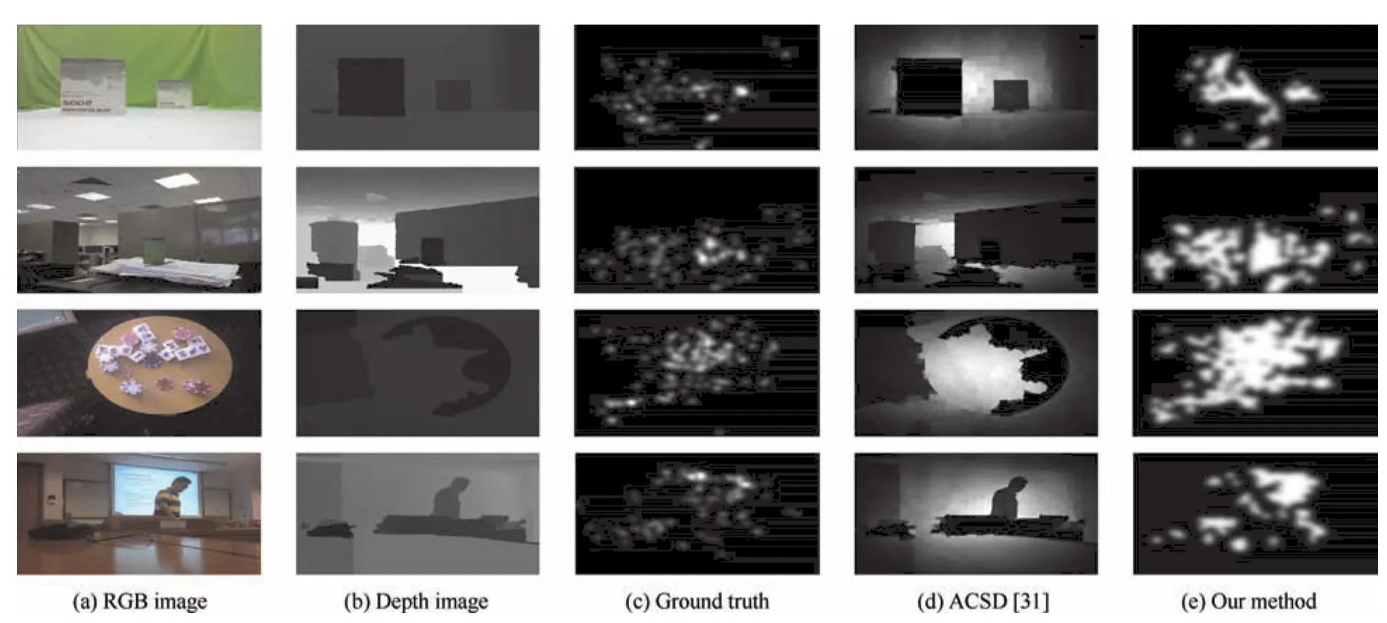
Fig.13.Visual comparison of saliency estimations of different 3D methods based on the NUS dataset.

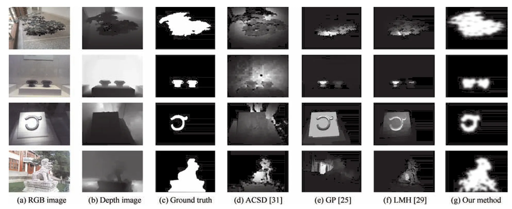
Fig.14. Visual comparison of saliency estimations of different 3D methods based on the NLPR dataset.

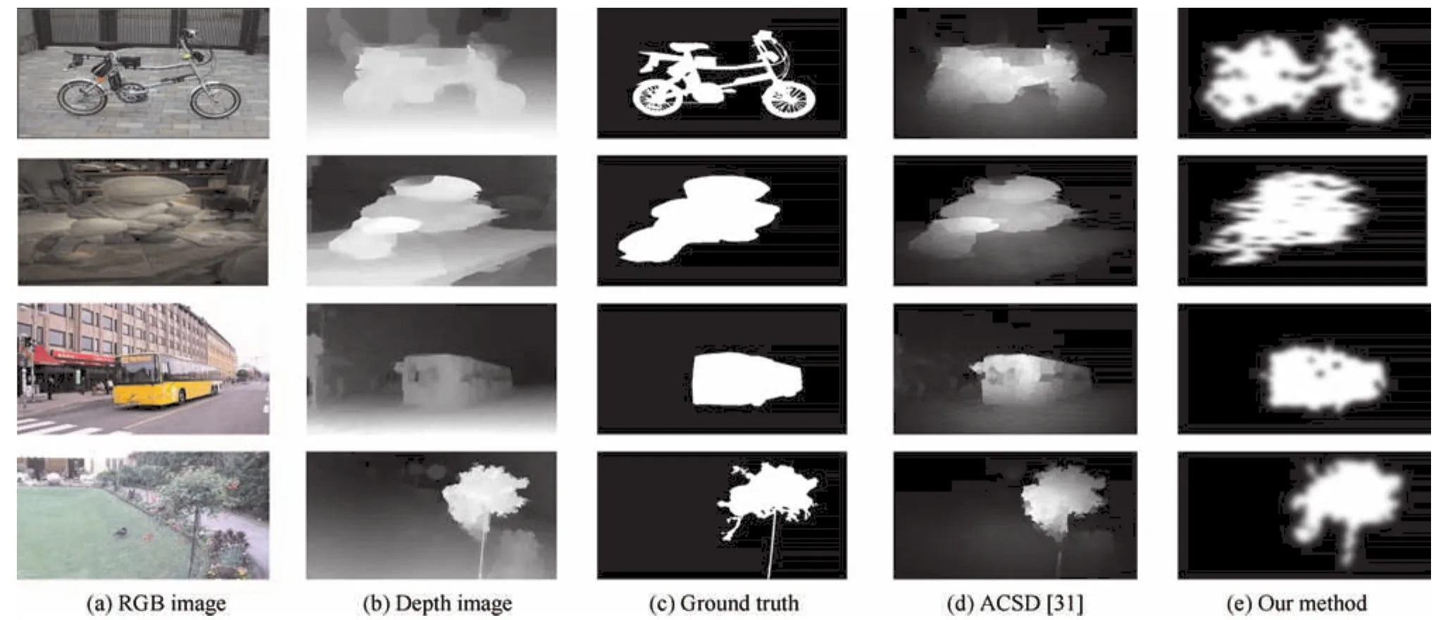
Fig.15.Visual comparison of the saliency estimations of different 3D methods based on the NJU-DS400 dataset.

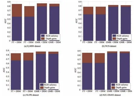
Fig.16. The quantitative comparisons of the performance of the depth cues.+indicates a linear combination strategy,and indicates a weighting method based on multiplication.

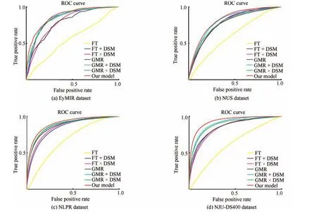
Fig.17. The quantitative comparisons of the performances of depth cues.+indicates a linear combination strategy,and indicates a weighting method based on multiplication.

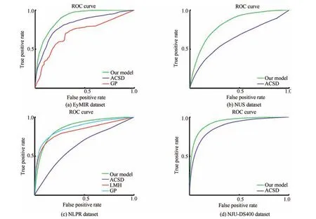
Fig.18.The ROC curves of different 3D saliency detection models in terms of the EyMIR dataset,NUS dataset,NLPR dataset and NJU-DS400.

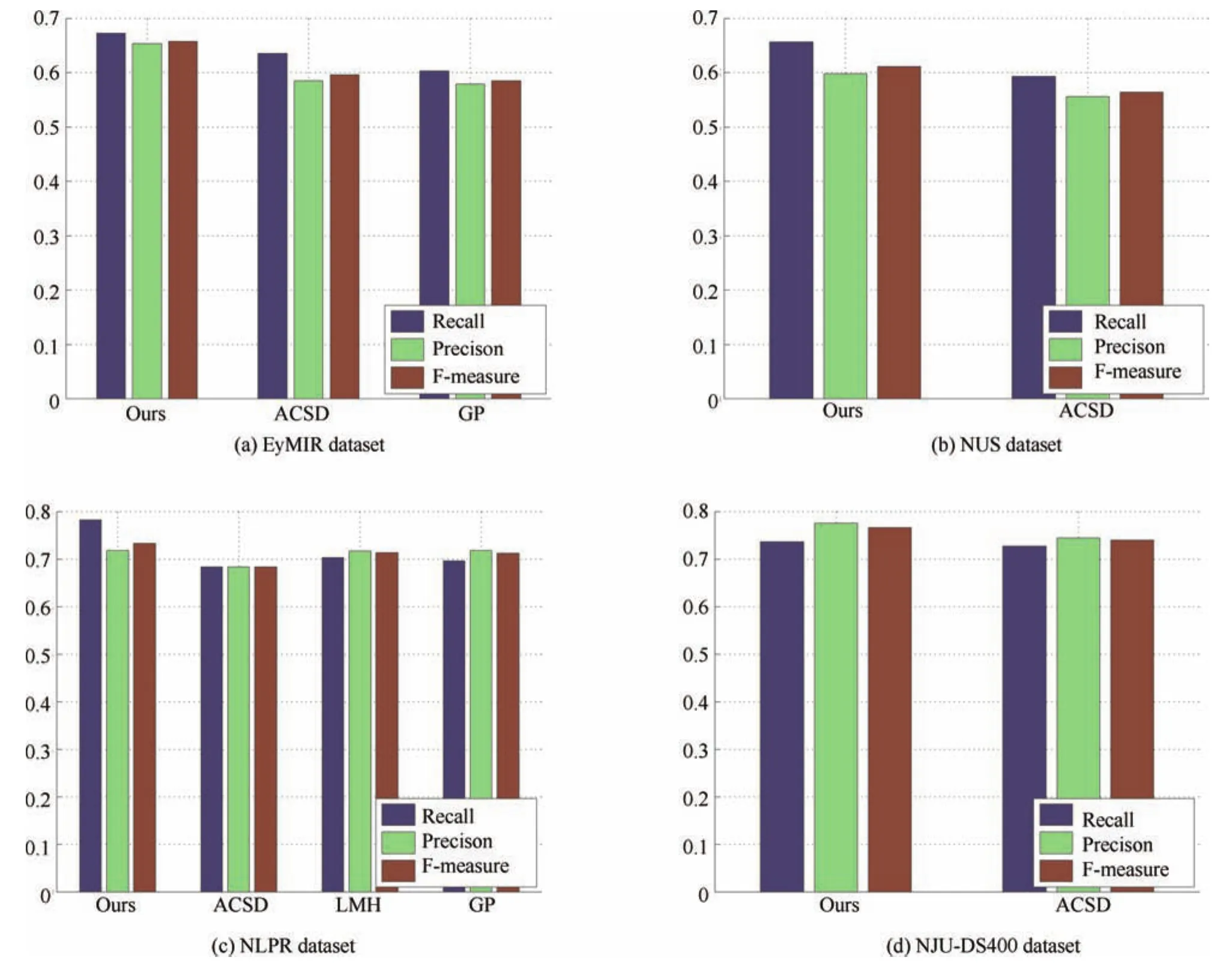
Fig.19.The F-measures of different 3D saliency detection models when used on the EyMIR dataset,NUS dataset,NLPR dataset and NJU-DS400.

4.3 Quantitative Evaluation

1)Comparison of the 2D Models Combined With DSM:In this experiment,we fi rst compare the performances of existing 2D saliency models before and after DSM fusing.We select two state-of-the-art 2D visual attention models:FT[5]and GRM[10].Figs.16 and 17 present the experimental results,where+and×denote a linear combination strategy and a weighting method,respectively.From Fig.16,we can see the strong in fl uence of using the DSM on the distribution of visual attention in terms of the viewing of 3D content.Although the simple late fusion strategy achieves improvements,it still suffers from inconsistency in the homogeneous foreground regions,which may be ascribed to treating the appearance and depth correspondence cues in an independent manner,as shown in Fig.11.We also provide the ROC curves for several compared methods in Fig.17.The ROC curves demonstrate that the proposed 3D saliency detection model performs better than the compared methods do.

2)Comparison of 3D Models:To obtain a quantitative evaluation,we compared ROC curves and F-measures from the EyMIR,NUS,NLPR and NJU-DS400 datasets.We compared the proposed model with the other existing models,i.e.,GP,LMH,and ACSD described in[25],[29]and[31],respectively.In this paper,the GP model,LMH model and ACSD model are classi fi ed as depth-pooling models.Figs.18 and 19 show the quantitative comparisons among these method on the constructed RGBD datasets in terms of ROC curves and F-measures.Methods such as[31]are not designed for such complex scenes but rather single dominant-object images.For the case that a single salient object is over an uninteresting background in the NJU-DS400 dataset,ACSD presented impressive results,as shown in Figs.18(d)and 19(d).In the NJU-DS400 dataset,we do not have experimental results for the LMH[29]and GP[25]methods due to the lack of depth information,which is required by their codes.

Due to the lack of global-context surface orientation priors in the EyMIR dataset,GP[25]is not able to apply the orientation prior to re fi ne the saliency detection,which has lower performance compared to the ACSD method,as shown in Figs.18(a)and 19(a).Interestingly,the LMH method,which uses Bayesian fusion to fuse depth and RGB saliency by simple multiplication,has lower performance compared to the GP method,which uses the Markov random fi eld model as a fusion strategy,as shown in Figs.18(c)and 19(c).However,LMH and GP achieve better perfor-mances than ACSD by using fusion strategies.The proposed RGBD method is superior to the baselines in terms of all the evaluation metrics.Although the ROC curves are very similar,Fig.19 shows that the proposed method improves the recall and F-measure when compared to LMH and GP,particularly in the NLPR dataset.This is mainly because the feature extraction using multi-scale superpixels enhances the consistency and compactness of salient patches.

3)Limitations:Because our approach requires training on large datasets to adapt to speci fi c environments,it has the problem that properly tuning the parameters for speci fi c new tasks is important to the performance of the DMNB model.The DMNB model does classi fi cation in one shot via a combination of mixed-membership models and logistic regression,where the results may depend on different choices ofK.The learned parameters will surely have good performances on the speci fi c stimuli but not necessarily on the new testing set.Thus,the weakness of the proposed methods is that to yield reasonable performances,we train our saliency model on the training set for speci fi cK.This problem could be addressed by using Dirichlet process mixture models to fi nd a properKfor new datasets.

5 Conclusion

In this study,we proposed a saliency detection model for RGB-D images that considers both color-and depth-based contrast features within a Bayesian framework.The experiments verify that the proposed model’s depth-produced saliency can serve as a helpful complement to the existing color-based saliency models.Compared with other competing 3D models,the experimental results based on four recent eye tracking databases show that the performance of the proposed saliency detection model is promising.We hope that our work is helpful in stimulating further research in the area of 3D saliency detection.

1 P.Le Callet and E.Niebur,“Visual attention and applications in multimedia technologies,”Proc.IEEE,vol.101,no.9,pp.2058−2067,Sep.2013.

2 A.Borji and L.Itti,“State-of-the-art in visual attention modeling,”IEEE Trans.Pattern Anal.Mach.Intell.,vol.35,no.1,pp.185−207,Jan.2013.

3 A.Borji,D.N.Sihite,and L.Itti,“Salient object detection:A benchmark,”inProc.12th European Conf.Computer Vision,Florence,Italy,2012,pp.414−429.

4 L.Itti,C.Koch,and E.Niebur,“A model of saliency-based visual attention for rapid scene analysis,”IEEE Trans.Pattern Anal.Mach.Intell.,vol.20,no.11,pp.1254−1259,Nov.1998.

5 R.Achanta,S.Hemami,F.Estrada,and S.Susstrunk,“Frequency-tuned salient region detection,” inProc.2009 IEEE Conf.Computer Vision and Pattern Recognition,Miami,FL,USA,2009,pp.1597−1604.

6 X.D.Hou and L.Q.Zhang,“Saliency detection:A spectral residual approach,”inProc.2007 IEEE Conf.Computer Vision and Pattern Recognition,Minneapolis,MN,USA,2007,pp.1−8.

7 J.Harel,C.Koch,and P.Perona,“Graph-based visual saliency,”inAdvances in Neural Information Processing Systems,Vancouver,British Columbia,Canada,2006,pp.545−552.

8 M.M.Cheng,G.X.Zhang,N.J.Mitra,X.L.Huang,and S.M.Hu, “Global contrast based salient region detection,”inProc.2011 IEEE Conf.Computer Vision and Pattern Recognition,Providence,RI,USA,2011,pp.409−416.

9 S.Goferman,L.Zelnik-Manor,and A.Tal,“Context-aware saliency detection,”inProc.2010 IEEE Conf.Computer Vision and Pattern Recognition,San Francisco,CA,USA,2010,pp.2376−2383.

10 C.Yang,L.H.Zhang,H.C.Lu,X.Ruan,and M.H.Yang,“Saliency detection via graph-based manifold ranking,”inProc.2013 IEEE Conf.Computer Vision and Pattern Recognition,Portland,OR,USA,2013,pp.3166−3173.

11 C.Y.Lang,T.V.Nguyen,H.Katti,K.Yadati,M.Kankanhalli,and S.C.Yan,“Depth matters:In fl uence of depth cues on visual saliency,”inProc.12th European Conf.Computer Vision,Florence,Italy,2012,pp.101−115.

12 K.Desingh,K.M.Krishna,D.Rajan,and C.V.Jawahar,“Depth really matters:Improving visual salient region detection with depth,”inProc.2013 British Machine Vision Conf.,Bristol,England,2013,pp.98.1−98.11.

13 J.L.Wang,Y.M.Fang,M.Narwaria,W.S.Lin,and P.Le Callet,“Stereoscopic image retargeting based on 3D saliency detection,”inProc.2014 IEEE Int.Conf.Acoustics,Speech and Signal Processing,Florence,Italy,2014,pp.669−673.

14 H.Kim,S.Lee,and A.C.Bovik,“Saliency prediction on stereoscopic videos,”IEEE Trans.Image Process.,vol.23,no.4,pp.1476−1490,Apr.2014.

15 Y.Zhang,G.Y.Jiang,M.Yu,and K.Chen,“Stereoscopic visual attention model for 3D video,”inProc.16th Int.Multimedia Modeling Conf.,Chongqing,China,2010,pp.314−324.

16 M.Uherˇc´ık,J.Kybic,Y.Zhao,C.Cachard,and H.Liebgott,“Line fi ltering for surgical tool localization in 3D ultrasound images,”Comput.Biol.Med.,vol.43,no.12,pp.2036−2045,Dec.2013.

17 Y.Zhao,C.Cachard,and H.Liebgott,“Automatic needle detection and tracking in 3D ultrasound using an ROI-based RANSAC and Kalman method,”Ultrason.Imaging,vol.35,no.4,pp.283−306,Oct.2013.

18 Y.M.Fang,J.L.Wang,M.Narwaria,P.Le Callet,and W.S.Lin, “Saliency detection for stereoscopic images,”IEEE Trans.Image Process.,vol.23,no.6,pp.2625−2636,Jun.2014.

19 A.Ciptadi,T.Hermans,and J.M.Rehg,“An in depth view of saliency,”inProc.2013 British Machine Vision Conf.,Bristol,England,2013,pp.9−13.

20 P.L.Wu,L.L.Duan,and L.F.Kong,“RGB-D salient object detection via feature fusion and multi-scale enhancement,”inProc.2015 Chinese Conf.Computer Vision,Xi’an,China,2015,pp.359−368.

21 F.F.Chen,C.Y.Lang,S.H.Feng,and Z.H.Song,“Depth information fused salient object detection,”inProc.2014 Int.Conf.Internet Multimedia Computing and Service,Xiamen,China,2014,pp.66.

22 I.Iatsun,M.C.Larabi,and C.Fernandez-Maloigne,“Using monocular depth cues for modeling stereoscopic 3D saliency,”inProc.2014 IEEE Int.Conf.Acoustics,Speech and Signal Processing,Florence,Italy,2014,pp.589−593.

23 N.Ouerhani and H.Hugli,“Computing visual attention from scene depth,”inProc.15th Int.Conf.Pattern Recognition,Barcelona,Spain,2000,pp.375−378.

24 H.Y.Xue,Y.Gu,Y.J.Li,and J.Yang,“RGB-D saliency detection via mutual guided manifold ranking,”inProc.2015 IEEE Int.Conf.Image Processing,Quebec City,QC,Canada,2015,pp.666−670.

25 J.Q.Ren,X.J.Gong,L.Yu,W.H.Zhou,and M.Y.Yang,“Exploiting global priors for RGB-D saliency detection,”inProc.2015 IEEE Conf.Computer Vision and Pattern Recognition Workshops,Boston,MA,USA,2015,pp.25−32.

26 H.K.Song,Z.Liu,H.Du,G.L.Sun,and C.Bai,“Saliency detection for RGBD images,”inProc.7th Int.Conf.Internet Multimedia Computing and Service,Zhangjiajie,Hunan,China,2015,pp.Atricle ID 72.

27 J.F.Guo,T.W.Ren,J.Bei,and Y.J.Zhu,“Salient object detection in RGB-D image based on saliency fusion and propagation,”inProc.7th Int.Conf.Internet Multimedia Computing and Service,Zhangjiajie,Hunan,China,2015,pp.Atricle ID 59.

28 X.X.Fan,Z.Liu,and G.L.Gun,“Salient region detection for stereoscopic images,”inProc.19th Int.Conf.Digital Signal Processing,Hong Kong,China,2014,pp.454−458.

29 H.W.Peng,B.Li,W.H.Xiong,W.M.Hu,and R.R.Ji,“Rgbd salient object detection:A benchmark and algorithms,”inProc.13th European Conf.Computer Vision,Zurich,Switzerland,2014,pp.92−109.

30 Y.Z.Niu,Y.J.Geng,X.Q.Li,and F.Liu,“Leveraging stereopsis for saliency analysis,”inProc.2012 IEEE Conf.Computer Vision and Pattern Recognition,Providence,RI,USA,2012,pp.454−461.

31 R.Ju,L.Ge,W.J.Geng,T.W.Ren,and G.S.Wu,“Depth saliency based on anisotropic center-surround difference,” inProc.2014 IEEE Int.Conf.Image Processing,Paris,France,2014,pp.1115−1119.

32 J.L.Wang,M.P.Da Silva,P.Le Callet,and V.Ricordel,“Computational model of stereoscopic 3D visual saliency,”IEEE Trans.Image Process.,vol.22,no.6,pp.2151−2165,Jun.2013.

33 I.Iatsun,M.C.Larabi,and C.Fernandez-Maloigne,“Visual attention modeling for 3D video using neural networks,”inProc.2014 Int.Conf.3D Imaging,Liege,Belgium,2014,pp.1−8.

34 Y.M.Fang,W.S.Lin,Z.J.Fang,P.Le Callet,and F.N.Yuan,“Learning visual saliency for stereoscopic images,” inProc.2014 IEEE Int.Conf.Multimedia and Expo Workshops,Chengdu,China,2014,pp.1−6.

35 L.Zhu,Z.G.Cao,Z.W.Fang,Y.Xiao,J.Wu,H.P.Deng,and J.Liu, “Selective features for RGB-D saliency,”inProc.2015 Conf.Chinese Automation Congr.,Wuhan,China,2015,pp.512−517.

36 G.Bertasius,H.S.Park,and J.B.Shi,“Exploiting egocentric object prior for 3D saliency detection,”arXiv preprint arXiv:1511.02682,2015.

37 H.H.Shan,A.Banerjee,and N.C.Oza,“Discriminative mixed-membership models,”inProc.2009 IEEE Int.Conf.Data Mining,Miami,FL,USA,2009,pp.466−475.

38 R.Achanta,A.Shaji,K.Smith,A.Lucchi,P.Fua,and S.S¨usstrunk,“SLIC superpixels compared to state-of-the-art superpixel methods,”IEEE Trans.Pattern Anal.Mach.Intell.,vol.34,no.11,pp.2274−2282,Nov.2012.

39 I.Rish, “An empirical study of the naive Bayes classi fi er,”J.Univ.Comput.Sci.,vol.3,no.22,pp.41−46,Aug.2001.

40 D.M.Blei and M.I.Jordan,“Variational inference for Dirichlet process mixtures,”Bayes.Anal.,vol.1,no.1,pp.121−143,Mar.2006.