Comparison of depth-averaged concentration and bed loadflux sediment transport models of dam-breakflow

Ji-heng Zho*,Ilhn ÖzgenDong-fng Ling,Reinhrd Hinkelmnn

aDepartment of Civil Engineering,Technische Universität Berlin,Berlin 13355,Germany

bDepartment of Engineering,University of Cambridge,Cambridge CB2 1PZ,UK

1.Introduction

Sediment transport inflowing water is one of the main factors in erosion and deposition processes.The mathematical and numerical modeling of these processes is challenging,because the erosion and deposition processes lead to a timevariable bottom elevation,which in return influences theflow.In addition,the sediment concentration is often considered to influence the momentum of the water.Furthermore,the erosion and deposition processes are usually described by empirical laws that depend on several parameters.

Guan et al.(2015)state that there are currently four types of sediment transport models.Two of them are so-called coupled models that solve the hydrodynamic and morphodynamic equations together.Based on the transport mode,coupled models can be categorized into the depth-averaged concentrationflux model(CF model)and the bed loadflux model(BF model).The other two types of models are so-called decoupled models,namely the two-layer transport model and the twophaseflow model.

In this paper,coupled models are considered.The BF model solves the depth-averaged shallow water equations together with the Exner equation,which describes the sediment transport based on bed load movement through a power law offlow velocity.The interaction between flow and sediment is accounted for by a variable parameter(Murillo and García-Navarro,2010).Existing literature about the Exnerequation treats the hydrodynamic and sediment mass conservation separately,without considering the influence of sediment movement on hydrodynamics(Soares-Fraz~ao and Zech,2011;Hudson and Sweby,2003;Liu et al.,2008;Liang,2011).This model assumes that the movement of the sediment is much slower than theflow velocity.The CF model describes the sediment transport as a fully mixed suspended load,while the erosion and deposition processes are calculated with empirical equations.The sediment is modeled as a concentration in the water column,and itsfluxes are calculated based on this concentration.Several additional parameters are introduced to calculate mass exchange between the dissolved sediment and the bed.In this study,source terms were introduced accounting for the interaction between the sediment andflow(Cao et al.,2004;Simpson and Castelltort,2006;Wu et al.,2012;Wu and Wang,2008).

The aim of this study was to compare the bed loadflux and depth-averaged concentrationflux sediment transport models for dam-breakflow over movable beds with regard to accuracy and suitable conditions for each model.

2.Governing equations

The coupled governing equations,consisting of the twodimensional shallow water equations and sediment transport,can be expressed as

where t is time;x and y are the two-dimensional Cartesian coordinates;q is the vector of conserved variables;f and g are theflux vectors of the conserved variables in the x-and ydirections,respectively;and the vector s represents the source terms.These vectors are expressed as

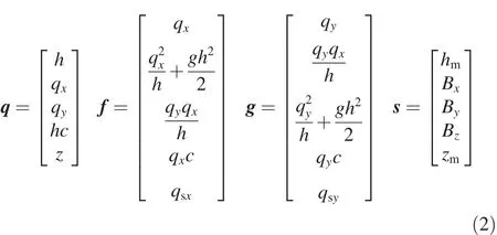
where h is the water depth;qxand qyare the unit-width discharges in the x-and y-directions,respectively,and qx=uh and qy=vh,with u and v being the depth-averaged velocity components in the x-and y-directions,respectively;z is the bottom elevation above the datum;c is theflux-averaged volumetric sediment concentration;g is the gravitational acceleration(9.81 m/s2);qsxand qsyare the sedimentfluxes in the x-and y-directions for the BF model,respectively,with the correspondingfluxes of the CF model described as qxc and qyc;hmis the mass source term offlow;Bxand Byare the momentum source terms in the x-and y-directions,respectively;Bzis the source term of the sediment concentration;and zmis the source term for the bottom elevation.By defining the flux and source terms associated with sediment transport,the BF or CF model can be obtained from Eq.(2).

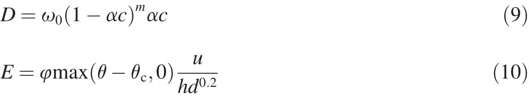
For the CF model,

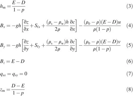
where p is the bed sediment porosity;Sfxand Sfyare the friction slopes in the x-and y-directions,respectively;E and D are substrate entrainment and depositionfluxes across the bottom boundary of flow,respectively; ρwand ρsare the density of water and sediment,respectively;ρ is the density of the sediment-water mixture,and ρ = ρw(1-c）+ ρsc;and ρ0is the density of the saturated bed,and ρ0= ρwp+ ρs(1-p）.These equations have been presented in Simpson and Castelltort(2006).

For the entrainment and deposition of sediment,this study used the following equations from Cao(1999):

where ω0is the settling velocity of a single particle in still water,and13.95ν/d; ν is the kinematic viscosity;d is the sediment diameter; the coefficient α is calculated by α =min[2.0，(1.0- φ）/c];m=2; φ is a calibration parameter;θ is the Shields parameter calculated by θ=u2/sgd,where s= ρs/ρw-1;and θcis the critical value of the Shields parameter for the initiation of sediment motion.

For the BF model,sedimentfluxes are calculated with Grass'model(Grass,1981)as follows:

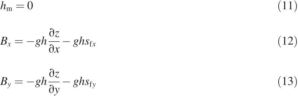
where ζ =1.0/(1.0-p）;and Agis an empirical coefficient that indicates the intensity of the interaction betweenflow and sediment,which is experimentally determined as a constant with a value between 0 and 1 s2/m.Details of the parameters can be found in Liang(2011).The BF model with the Exner equation is known to overestimate theflow velocity because sediment particles do not influence the momentum of thefluid.Extending the momentum source terms of the BF model with-ψsqsxand-ψsqsyin the x-and y-directions,respectively,is proposed,in order to account for momentum losses due to the sediment movement.As the influence of these source terms on the eigen-structure of the governing equations has been neglected,the calibration coefficient ψ is introduced.

3.Numerical methods

For both models,a cell-centered Godunov-type scheme is used for solving the equations,and a second-order monotonic upstream-centered scheme for conservation laws(MUSCL)(van Leer,1979)is employed to reconstruct the value at the middle point of the edge.To preserve the non-negative water depth and the C-property(Gallardo et al.,2007),the hydrostatic reconstruction method(Audusse et al.,2004)is used.A total variation diminishing scheme presented in Hou et al.(2013b)is applied to avoid spurious oscillations.

In the CF model,the numericalfluxes are calculated by the Harten,Lax,and van Leer approximate Riemann solver with the contact wave restored(HLLC)(Toro et al.,1994).In the BF model,the additionalfluxes qsxand qsychange the eigenstructure of the governing equations.Thus,the modified HLLCflux calculation method by Liang(2011)is used in this model.

A two-stage Runge-Kutta scheme is applied for the time discretization.

3.1.Treatment of source terms

In sediment transport models,the influence of sediment movement is reflected by source terms.For shallow water equations,the friction source terms are evaluated with a splitting point-implicit method(Bussing and Murman,1988).

Valiani and Begnudelli(2006)presented an efficient divergence form for the slope source term calculation and Hou et al.(2013a)modified this slope source term treatment to obtain higher-order accuracy for the bed slope source term in the classical shallow water model.Based on this method,a modified source term treatment was derived in this study,induced by the waterflow density change.It is noted that this treatment requiresflow with density change,which means that the volumetric concentration is a necessary condition,or,in other words,this method cannot be applied to the BF model.

In a one-dimensional case,the source terms in the CF model related to gravity force can be written in the integral form as follows:

where Bgxis the gravity source term,and Ω is the control volume.Source terms related to the gravity force are divided into the bed slope source term of theflow and the gradient source term of the sediment concentration.This assumes that sediment concentration andflow depth are independent of each other.The source terms are calculated separately with one of the two values remaining constant.

The derivation process will not be shown in detail here.The overall derivation for a bed slope can be found in Hou et al.(2013a),and the application of the method to the source terms in Eq.(18)is

where Fs(q）denotes theflux of the slope source term;nfxand nfyare the components of the outward unit normal vector nfalong the x-and y-directions,respectively,of the considered face;hM,zbM,ρM= ρw(1-cM）+ ρscM,and cMrepresent the water depth,bottom elevation,density,and concentration at the centroid of the considered cell,respectively;and hf,zbf,ρf= ρw(1-cf）+ ρscf,and cfrepresent the corresponding values for the face.The integral of slope source sbover a cell can be rewritten as

where k and neare the index and the number of the edges in the considered cell,respectively.

3.2.Main procedure of models'application

The models use a ghost cell treatment to impose boundary conditions(LeVeque,2002).The updating procedure of the models can be summarized in the following steps:

Step 1:Update the ghost cells.

Step 2:Interpolate the edge values by means of the MUSCL reconstruction from Hou et al.(2013b).

Step 3:Carry out the hydrostatic reconstruction(Audusse et al.,2004).

Step 4:Use the novel slope source treatment to calculate the divergence form of the bed and density slope source terms for the CF model and use the divergence form to calculate the bed slope source terms while neglecting the density change with regard to ρf/ρM=1 for the BF model,then calculate interfacefluxes of mass and momentum in the same loop with the slope sourcefluxes,with different HLLC approximate solvers for the CF and BF models.

Step 5:Calculate source terms that are evaluated based on cell values.

Step 6:Calculate the intermediate values of cells.

Step 7:Carry out the Runge-Kutta time integration by repeating steps 1 through 6 using the intermediate values.

4.Test cases

In this section,two test cases are presented.Thefirst case is a one-dimensional dam-breakflow over a movable bed.The second case is dam-breakflow over variable bed topography.4.1.Error calculation

The volume weighted L1-norm(Sun and Takayama,2003)was used to quantify the difference between results:

where NCis the total number of the cells,i is the cell index,Aiis the area of the computational cell i,qiis the exact solution of the computational cell i,and q′is the numerical solution.

4.2.One-dimensional dam-breakflow over movable bed

This test case was initially presented by Cao et al.(2004),who described a numerical solution for reference.The domain was 4000 m long.A dam was set up at a position of 2000 m.The water surface elevation on the left side of the dam was 40 m,and the water surface elevation on the right side of the dam was 2 m.The sensitivity of Manning's coefficient,sediment diameters,and sediment porosity were investigated.

This case used the same parameters as Cao et al.(2004)to verify the model.This case was also used as the reference case for the sensitivity study.The parameters were as follows:the diameter of the bed sediment was set to 8 mm,the porosity of the bed sediment was 0.4,and the density of the sediment was 2650 kg/m3.The calibration parameter was set to φ=0.015 in the CF model.The modified source term in the BF model was omitted,i.e.,ψ=0,to demonstrate the overestimation of velocities by the BF model.Results are shown in Fig.1.While the CF model shows strong agreement with the results reported in Cao et al.(2004),the BF model results do not agree.This is expected,as the CF model uses similar model concepts to the model by Cao et al.(2004),i.e.,suspended load transport that influences the momentum balance,while in the BF model the sediment is transported solely as bed load,i.e.,the sediment is not transported as suspended load.Thus,the immediate change in the bottom elevation in the BF model is described by the sediment concentration in the CF model.Therefore,the BF model overestimates the erosion upstream and the deposition downstream.It can be argued that the CF model captures the physical process better,as the results seem to agree with the experimental results of Spinewine and Zech(2007),who replicated this test case in a laboratory.It is noted that,in reality,distinguishing suspended load from bed load is not trivial.

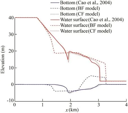
Fig.1.Comparison of water surface elevations and bottom elevations of BF model and CF model after 60 s.

In addition,as discussed in Audusse et al.(2012),using Ag=0.2 s2/m for unsteadyflow will lead to almost constant water level downstream,which might also explain the greater deviation of the BF model,and because the influence from the sediment movement has been neglected,the water level wave front of the BF model is significantly faster than that of the CF model.Fig.2 shows the unit-width discharge distribution in the domain.It is noted that the BF model tends to overestimateflow velocities,because the sediment movement does not influence the fluid dynamics.

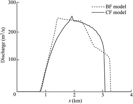
Fig.2.Unit-width discharge after 60 s.

Fig.3.Comparison of water surface elevations and bottom elevations of modified BF model and CF model after 60 s.

To capture the shock wave position downstream,the coefficient ψ of the BF model was set to 0.05.A comparison between the CF model and the modified BF model is shown in Fig.3.After both models were verified,a sensitivity analysis was carried out.Manning's coefficient,the sediment diameter,and the sediment porosity were varied and their respective influences on the results were quantified by means of the L1-norm of the bottom elevation with regard to the reference case.In each simulation run,one parameter was increased or decreased by 50%of itself,while the values of all other parameters were the same as those in the reference case.The results are summarized in Table 1.The results for varying Manning's coefficient are shown in Fig.4.Increasing friction causes different types of erosion.In the BF model,Manning's coefficient is not considered in the sediment movement process,so the friction only decreases theflow velocity,which leads to less erosion.In contrast,with an increasing friction parameter in the CF model,θ will grow larger,causing more erosion.

For the CF model,Manning's coefficient and the sediment porosity show an almost linear relationship with the change of bottom elevation.For the BF model,the sediment porosity is identified as the most sensitive parameter.This is partly because the BF model in this study used a constant Agto calculate the sedimentflux and Manning's coefficient was not used.

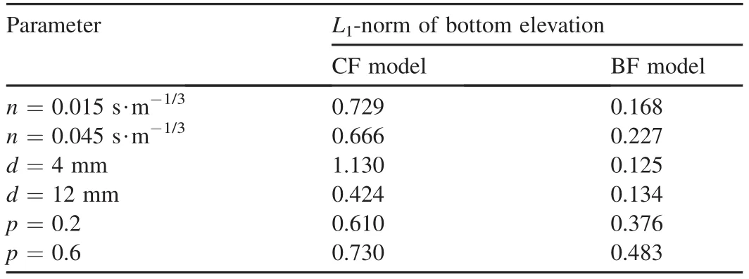
Table 1 L1-norm summary of bottom elevation in dependency of model parameters.

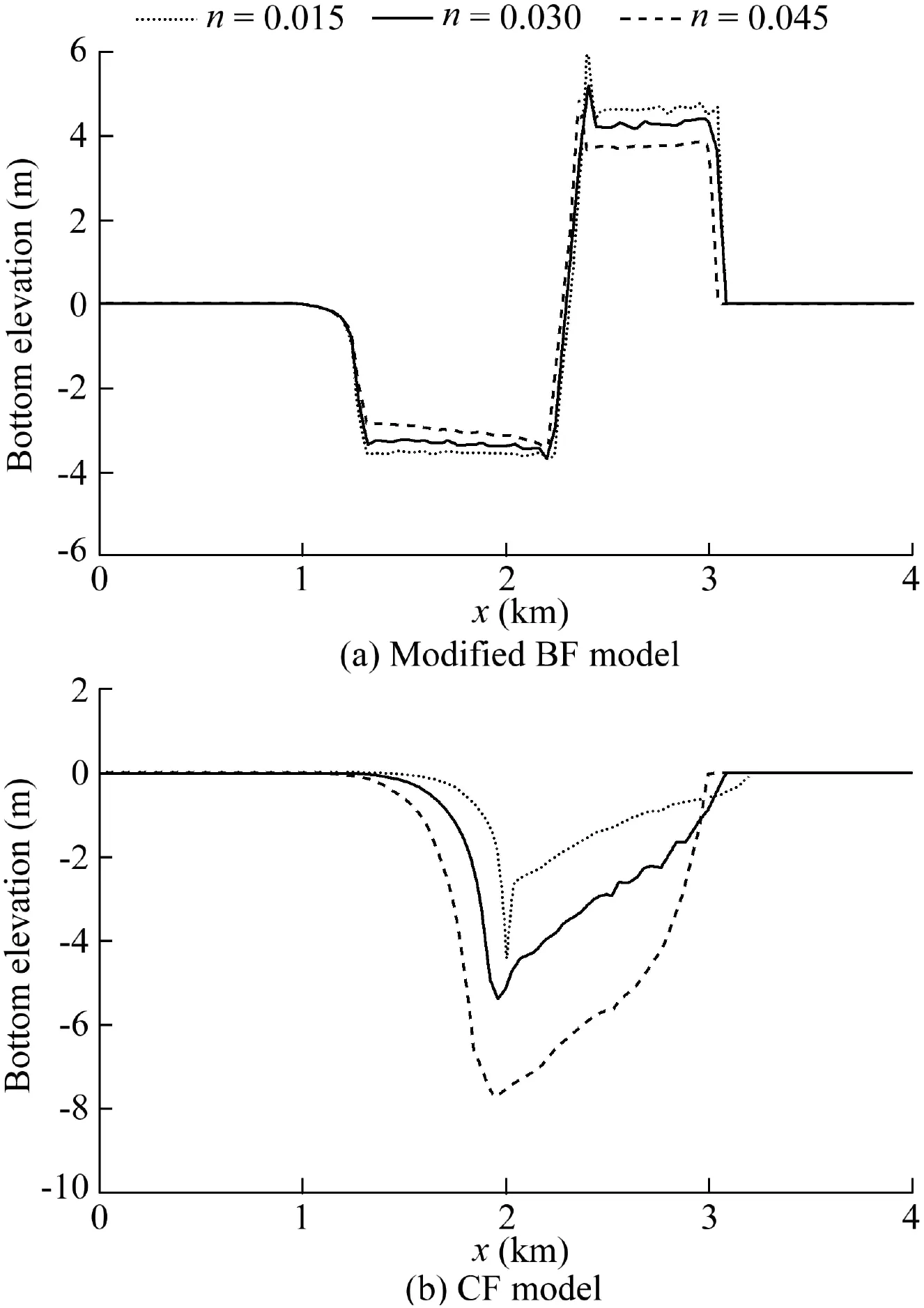
Fig.4.Comparison of results with varying Manning's coefficient for modified BF model and CF model.

4.3.Simulation of laboratory dam-break experiment over movable discontinuous bottom

Dam-break experiments over movable beds were carried out at the laboratory of the Department of Civil and Environmental Engineering at Universit′e Catholique de Louvain,Belgium,by Spinewine(2005).In comparison to the previous example,the bottom topography in these cases was more complex,as initial discontinuities were introduced in the initial domain.

The domain was a rectangular glassflume,which was 6 m long,0.25 m wide,and 0.70 m high.At the middle of theflume there was a thin gate that simulated the dam.Sand bed material had a uniform diameter,d=1.82 mm,sediment density was ρs=2683 kg/m3,and porosity was p=0.47.Different initial conditions were imposed by adjusting the initial water depth and thickness of the bed material upstream and downstream of the gate.All four scenarios had the sameupstream water surface elevation of 0.35 m and downstream bottom elevation of 0 m.The upstream bed elevation and the downstream water surface elevation for the four scenarios are shown in Table 2.A detailed discussion of the experiments can be found in El Kadi Abderrezzak and Paquier(2011).

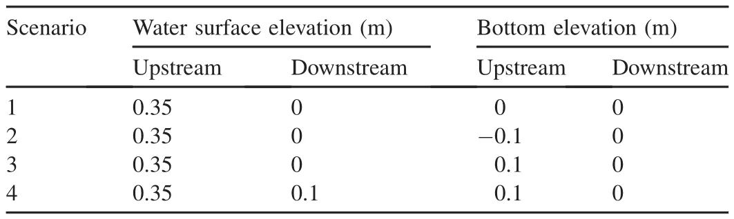
Table 2 Upstream and downstream elevations for four scenarios.

The experimental results were replicated with both models,in order to study the applicability of both models in different scenarios with complex topography.

For the BF model,Agwas set to 0.0006.This is because the water depth here was comparably low,implying less interaction between flow and sediment.The parameter ψ was set to 0.1 for theflow momentum source term dealing with the sediment movement.For the CF model,φ was set to 0.002.The results for scenarios 1,2,3,and 4 are plotted in Fig.5,in which the experimental data are from Spinewine(2005).

As shown in Fig.5,for scenarios 1 and 2,both the modified BF model and the CF model show strong agreement with the experimental data for the bottom elevation.The agreement of the water surface elevation is poor for both models,but the location of the shock is captured accurately.The deviation between the models and experiments might be due to the mathematical model limitations of the shallow water equations,which cannot account for the non-hydrostatic pressure distribution that is expected at the beginning of a dam break.For scenario 1,the CF model provides better results than the modified BF model.The reason for this is the same as in thefirst test case,i.e.,the sediment in the CF model is still dissolved in the fluid while the modified BF model causes immediate deposition.The CF model has stiff source terms,i.e.,for cases with dry beds,the erosion rate goes to infinity.As a numerical treatment,if the water depth is less than the sediment diameter,the erosion rate is set to zero.This enables a robust simulation of sediment transport on a dry bed.For scenario 2,both models provide about the same agreement for the bottom elevation.However,the modified BF model shows better agreement with the experimental data for water surface elevation.

Fig.5.Water surface elevation and bottom elevation at t=1.247 s for different scenarios.

The results for scenario 3 show that the modified BF model provides better agreement for the bottom elevation.Both models fail to capture the shock properly.For the water surface elevation,the modified BF model results may be considered better.For scenario 4,the modified BF model provides strong agreement for the bottom elevation.The water surface elevation could not be reproduced by either of the models,but the modified BF model provides better agreement.The shock is again not captured properly.It can be concluded that the sharply descending bottom is numerically more challenging for both models and leads to errors in the hydrodynamics and morphodynamics.The shock cannot be captured accurately in these cases.For theflat bottom and the sharply ascending bottom,these errors are not observed;the shock is captured accurately.

Overall,the results are comparable to the ones reported in El Kadi Abderrezzak and Paquier(2011).

5.Conclusions

A bed loadflux(BF)model and a depth-averaged concentrationflux(CF)model were used to simulate sediment transport in two different ways:as bed load and as suspended load.The bottom change in the BF model is calculated using the sedimentflux of the bed load.Therefore,the morphodynamics are instantaneous.In contrast,in the CF model,the sediment transport is a process that depends on the entrainment and deposition that are calculated separately using empirical formulas.The water carries the sediment and the sediment particle movement influences the water momentum.Thus,the CF model concept is more complex than the BF model concept.

A simple heuristic modification is proposed that introduces additional source terms to the momentum balance.A modified bed slope source term treatment that considers the density change of theflow in the CF model meant to obtain higherorder accuracy,is presented in this paper.

Two test cases were described that compare the BF model with the CF model.In thefirst test case,both models were verifiedbycomparisonwithresultsfromCaoetal.(2004).After the verification,a sensitivity test was carried out for different parameters.For the CF model,Manning's coefficient and the sediment porosity show an almost linear relationship with the bottom change.For the BF model,the sediment porosity is considered the most sensitive parameter.The influence of the friction in both models shows the opposite impact.

In the second test case,the modified BF model and the CF model were compared with experimental data.The BF and CF models both provide good results for the morphodynamics,but for the water surface,the numerical models show greater water depth in the wave front,which might result from nonhydrostaticflow conditions in the experiment.However,in the investigated cases,the sediment movement and its influence on the water surface elevation were relatively small,so that both models lead to similar surface water levels.For realworld applications such as realflood events,the difference between the morphodynamics may lead to larger differences in the water surface levels.

The empirical coefficient ψ in the BF model will be investigated in the future.It can be concluded that the modified BF model can be used for sediment transport modeling for relatively steadyflow,and the CF model can be used for unsteadyflow.However,it is acknowledged that in practice it is difficult to separate these cases.

Audusse,E.,Bouchut,F.,Bristeau,M.O.,Klein,R.,Perthame,B.,2004.A fast and stable well-balanced scheme with hydrostatic reconstruction for shallow waterflows.SIAM J.Sci.Comput.25(6),2050-2065.https://doi.org/10.1137/S1064827503431090.

Audusse,E.,Berthon,C.,Chalons,C.,Delestre,O.,Goutal,N.,Jodeau,M.,Sainte-Marie,J.,Giesselmann,J.,Sadaka,G.,2012.Sediment transport modelling:Relaxation schemes for Saint-Venant-Exner and three layer models.ESAIM:Proc.Surv.38,78-98.https://doi.org/10.1051/proc/201238005.

Bussing,T.R.,Murman,E.M.,1988.Finite-volume method for the calculation of compressible chemically reactingflows.AIAA J.26(9),1070-1078.https://doi.org/10.2514/3.10013.

Cao,Z.X.,1999.Equilibrium near-bed concentration of suspended sediment.J.Hydraul.Eng.125(12),1270-1278.https://doi.org/10.1061/(ASCE)0733-9429(1999)125:12(1270).

Cao,Z.X.,Pender,G.,Wallis,S.,Carling,P.,2004.Computational dam-break hydraulics over erodible sediment bed.J.Hydraul.Eng.130(7),689-703.https://doi.org/10.1061/(ASCE)0733-9429(2004)130:7(689).

El Kadi Abderrezzak,K.,Paquier,A.,2011.Applicability of sediment transport equilibrium formulas to dam-breakflows over movable beds.J.Hydraul.Eng.137(2),209-221.https://doi.org/10.1061/(ASCE)HY.1943-7900.0000298.

Gallardo,J.M.,Carlos,P.,Manuel,C.,2007.On a well-balanced high-orderfinite volume scheme for shallow water equations with topography and dry areas.J.Comput.Phys.227(1),574-601.https://doi.org/10.1016/j.jcp.2007.08.007.

Grass,A.J.,1981.Sediment Transport by Waves and Currents.University College and Department of Civil Engineering,London.

Guan,M.F.,Wright,N.G.,Sleigh,P.A.,2015.Multimode morphodynamic model for sediment-ladenflows and geomorphic impacts.J.Hydraul.Eng.141(6),1-24.https://doi.org/10.1061/(ASCE)HY.1943-7900.0000997.

Hou,J.M.,Liang,Q.H.,Simons,F.,Hinkelmann,R.,2013a.A 2D wellbalanced shallowflow model for unstructured grids with novel slope source term treatment.Adv.Water Resour.52,107-131.https://doi.org/10.1016/j.advwatres.2012.08.003.

Hou,J.M.,Simons,F.,Hinkelmann,R.,2013b.A new TVD method for advection simulation on 2D unstructured grids.Int.J.Numer.Meth.Fluid.71(10),1260-1281.https://doi.org/10.1002/fld.3709.

Hudson,J.,Sweby,P.K.,2003.Formulations for numerically approximating hyperbolic systems governing sediment transport.J.Sci.Comput.19(1-3),225-252.https://doi.org/10.1023/A:1025304008907.

LeVeque,R.J.,2002.Finite Volume Methods for Hyperbolic Problems.Cambridge University Press,New York.https://doi.org/10.1017/CBO9780 511791253.

Liang,Q.H.,2011.A coupled morphodynamic model for applications involving wetting and drying.J.Hydrodyn.Ser.B 23(3),273-281.https://doi.org/10.1016/S1001-6058(10)60113-8.

Liu,X.,Landry,B.J.,Garcia,M.H.,2008.Two-dimensional scour simulations based on coupled model of shallow water equations and sediment transport on unstructured meshes.Coast Eng.55(10),800-810.https://doi.org/10.1016/j.coastaleng.2008.02.012.

Murillo,J.,García-Navarro,P.,2010.An exner-based coupled model for twodimensional transientflow over erodible bed.J.Comput.Phys.229(23),8704-8732.https://doi.org/10.1016/j.jcp.2010.08.006.

Simpson,G.,Castelltort,S.,2006.Coupled model of surface waterflow,sediment transport and morphological evolution.Comput.Geosci.32(10),1600-1614.https://doi.org/10.1016/j.cageo.2006.02.020.

Soares-Fraz~ao,S.,Zech,Y.,2011.HLLC scheme with novel wave-speed estimators appropriate for two-dimensional shallow-waterflow on erodible bed.Int.J.Numer.Meth.Fluid.66(8),1019-1036.https://doi.org/10.1002/fld.2300.

Spinewine,B.,2005.Two-layer Flow Behaviour and the Effects of Granular Dilatancy in Dam-break Induced Sheet-flow.Ph.D.Dissertation.Universit′e catholique de Louvain,Louvain.

Spinewine,B.,Zech,Y.,2007.Small-scale laboratory dam-break waves on movable beds.J.Hydraul.Res.45(s1),73-86.https://doi.org/10.1080/00221686.2007.9521834.

Sun,M.,Takayama,K.,2003.Error localization in solution-adaptive grid methods.J.Comput.Phys.190(1),346-350.https://doi.org/10.1016/S0021-9991(03)00278-X.

Toro,E.F.,Spruce,M.,Speares,W.,1994.Restoration of the contact surface in the HLL-Riemann solver.Shock Waves 4(1),25-34.https://doi.org/10.1007/BF01414629.

Valiani,A.,Begnudelli,L.,2006.Divergence form for bed slope source term in shallow water equations.J.Hydraul.Eng.132(7),652-665.https://doi.org/10.1061/(ASCE)0733-9429(2006)132:7(652).

van Leer,B.,1979.Towards the ultimate conservative difference scheme.V.A second order sequel to Godunov's method.J.Comput.Phys.32,101-136.https://doi.org/10.1016/0021-9991(79)90145-1.

Wu,W.,Wang,S.S.,2008.One-dimensional explicitfinite-volume model for sediment transport.J.Hydraul.Res.46(1),87-98.https://doi.org/10.1080/00221686.2008.9521846.

Wu,W.,Marsooli,R.,He,Z.,2012.Depth-averaged two-dimensional model of unsteadyflow and sediment transport due to noncohesive embankment break/breaching.J.Hydraul.Eng.138(6),503-516.https://doi.org/10.1061/(ASCE)HY.1943-7900.0000546.