Wave propagation speeds and source term influences in single and integral porosity shallow water equations

Ilhn Özgen*,Ji-heng ZhoDong-fng Ling,Reinhrd Hinkelmnn

aDepartment of Civil Engineering,Technische Universit¨at Berlin,Berlin 13355,Germany

bDepartment of Engineering,University of Cambridge,Cambridge CB2 1PZ,UK

1.Introduction

Urbanflooding is a multiscale process.An urban catchment might span several hundreds of square kilometers,and individual buildings usually span up to a hundred square meters.The interaction between individual buildings or building blocks and theflood wave,occurring at the building scale,is the most significant process influencing the entire flow field.

Using a two-dimensional shallow water model,or a simplified form of it,to model urban flooding is considered the state-of-the-artmethodology.In classicalshallow water models,buildings have to be explicitly discretized either by increasing the bed elevation accordingly or by removing the corresponding areas from the computational mesh(Schubert and Sanders,2012).In both cases,the mesh has to be locally refined near the buildings,which results in high numbers of cells.In recent years,explicit Godunov-type methods have attracted increasing interest as applied to such tasks,because of their attractive numerical properties(shockcapturing,monotonicity preserving,and the ability to deal with wet/dry fronts and transcriticalflow).The high computational cost of these types of methods,combined with high numbers of cells leads to a huge CPU requirement that is classically approached by means of parallel computation techniques(Hinkelmann,2005).

The so-called macroscopic modeling of urbanfloods is an alternative approach,in which the catchment is discretized using a coarser resolution than the building scale,i.e.,the size of the cell is larger than that of the building,and conceptual approaches are used to describe certain hydraulic properties of the urban catchment.Typically,porosity terms are used to account for the presence of buildings inside a computational cell without explicitly discretizing them.These equations are then referred to as porosity shallow water equations(PSWEs).Inspired by the pioneering work in Defina(2000),Guinot and Soares-Fraz~ao(2006)derived the single porosity shallow water model(SP model),which uses a single porosity defined inside the cell to account for reductions in storage and conveyance.Sanders et al.(2008)derived an integral porosity model,also referred to as the anisotropic porosity shallow water model(AP model),where the storage reduction is accounted for with a porosity term defined inside the cell and the conveyance reduction is accounted for with a porosity term at the cell edges.In¨Ozgen et al.(2016a,2016b),water depthdependent porosities were derived to enable full inundation of sub-grid elements.

Guinot and Soares-Fraz~ao(2006)as well as Mohamed(2014)have shown that the wave propagation speeds of the SP model are the same as those of the classical shallow water equations.As shown in Guinot et al.(2017),the wave propagation speeds of the AP model differ from those of the classical shallow water equations and the SP model,and thesefindings are supported by numerical experiments conducted in¨Ozgen et al.(2016b).In addition,different source terms arise in the SP model and the AP model.Recently,Ferrari et al.(2017)derived an augmented Roe scheme for the SP model that incorporates the source term in the Riemann problem.

In this study,the implications of the differences in wave propagation speeds and source terms between the SP model and the AP model were analyzed,using a methodology described in Murillo et al.(2007).The governing equations of the SP model and the AP model are presented,accompanied by an eigenvalue analysis for each mathematical model.Then,the influences of the wave propagation speeds and the source terms on the stability of each model are analyzed.Finally,computational tests for investigation of the influences of the wave propagation speeds and source terms on the model results are described.

2.Governing equations

2.1.Single porosity shallow water equation

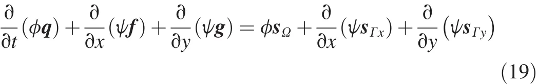
The single PSWE,i.e.,the SP model,is written in the vector form as follows:

where t is time;x and y are the axes in the Cartesian coordinate system;φ is the storage porosity expressing the fraction of the control volume that is not occupied by structures;q is the vector of conserved variables;f and g are theflux vectors in the x-and y-directions,respectively;sΩis the source term in the control volume;and sφis the porosity source term that describes the momentum variation due to the variation in porosity.The vectors are defined as follows:

where h is the water depth;u and v are the velocities in the xand y-directions,respectively;g is the acceleration due to gravity;sgxand sgyare the geometric source terms in the x-and y-directions,respectively;and sfxand sfyare the friction source terms in the x-and y-directions,respectively.

The source term sΩdescribes two separate processes:the momentum variation due to the gravity,which can be calculated as follows:

where z is the bed elevation;and the momentum variation due to friction and drag,which can be calculated using Manning's law:

The derivation of Eq.(1)through(4),initially presented in Guinot and Soares-Fraz~ao(2006),is based on homogenizing heterogeneities inside a control volume,expressed with a single variable φ,which implies the assumption of a representative elementary volume(REV).As discussed in Guinot(2012),the existence of such an REV in the urban area is controversial but has no consequences with regard to the applicability of the equations.

An eigenvalue analysis ofthe homogeneous,onedimensional version of Eq.(1),i.e.,

is presented in Mohamed(2014)and Guinot et al.(2017).Eq.(7)is linearized as follows:

where A is the Jacobian matrix,which is calculated as follows:

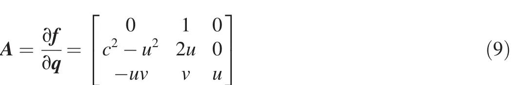
with c being the wave celerity,and

The real and distinct eigenvalues of Eq.(7)are then determined to be

which are the same as those of the classical shallow water equations(LeVeque,2002).Consequently,the right eigenvectors of Eq.(1)are also identical to those of the classical shallow water equations:

In Mohamed(2014),Eq.(1)was augmented with an additional equation:

which yields the fourth eigenvalue,λ4=0,for a stationary wave,associated with the variable φ.

2.2.Integral porosity shallow water equation

The limitation of the SP model is its inability to represent directionality and blocking effects(Guinot,2012).In order to overcome this limitation,an integral form of PSWEs was presented in Sanders et al.(2008),which uses a storage porosity defined inside the control volume to account for the reduction in storage and a conveyance porosity defined at the edge of the control volume to account for the reduction in conveyance.In the literature,these equations are referred to as the anisotropic or integral PSWEs.

As these equations are in the integral form,discontinuous solutions are allowed and there is no need for an REV assumption for the derivation.Porosities are calculated by means of a phase function φ(x,y)that is 1 if the evaluation point(x,y)corresponds to a void and 0 if it corresponds to an obstacle.Then,the storage porosity is calculated as follows:

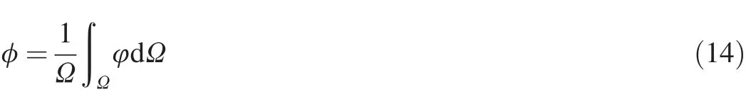
and the conveyance porosity is calculated as follows:

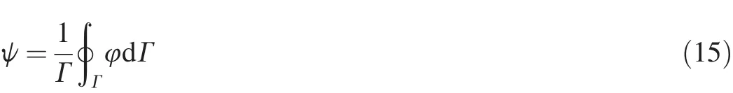
with Ω being the control volume,and Γ being the boundary of the control volume.

The AP model is written in the vector form as follows:

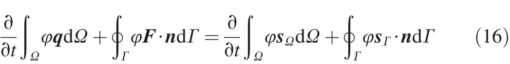
with F being theflux tensor,n being the unit normal vector pointing outwards from the control volume,and sΓbeing the source term at the boundary,which arises due to unresolved solid-fluid interface pressures(Bird et al.,2007).q and sΩare defined in Eqs.(2)and(4),and F and sΓare written as follows:

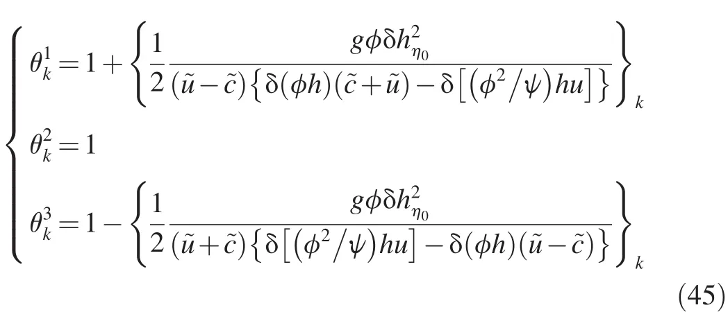
where hη0represents the water depth inside the cell,evaluated for a constant average water level elevation η0inside the control volume.Carrying out discretized integral of the individual terms in Eq.(16)and using Eqs.(14)and(15)provide the following:

where ljis the length of the jth boundary edge,and s stands for a suitable integration of the source terms sΩand sΓ.The integral over the boundary in Eq.(16)has been replaced by a sum over j discrete boundary edges.Eq.(18)is essentially afinite volume discretization,and indeed,because Eq.(16)is only meaningful in the integral form,it can only be solved by means of afinite volume method.

Going back to Eq.(16),under the assumption that the solution is sufficiently smooth,the control volume can be made infinitesimally small.Applying the Green-Gauß theorem yields the differential form of the AP model.This technique has been applied in Sanders et al.(2008),where it is shown that in the context of an infinitesimally small control volume,the storage porosity φ equals the conveyance porosity ψ,and the AP model is made equivalent to the SP model.Based on the discussion in Guinot et al.(2017),for the sake of argument,the porosity terms are not set to be equal,which then,after algebraic manipulation,leads to the following differential form of the AP model:

where f and g are identical to the flux vectors in Eq.(1),and sΩis identical to the source term presented in Eq.(4).The boundary source terms sΓxand sΓyare the first and second columns of sΓand replace the source term sφin Eq.(1).

It is perhaps interesting to note that a source term similar to sφappears in the cross-section-averaged Saint-Venant equations due to channel narrowing,which,through Leibniz's rule for differentiation under the integral sign,can be transformed into a form similar to sΓ(Cunge et al.,1980).

Considering again only the homogeneous part of the onedimensional form of Eq.(19),i.e.,

and linearizing Eq.(20)provide the following:

with the Jacobian matrix B defined as

The real and distinct eigenvalues of Eq.(20)are calculated as

which differ from those in the SP model(Eq.(11))by the factor ψ/φ.Guinot et al.(2017)note that if ψ/φ ＞1,the wave propagation speeds of the AP model are larger than those of the classical shallow water model.This would imply that the presence of the conveyance porosity increases the wave propagation speed,which is physically not meaningful.The right eigenvectors of Eq.(19)are obtained,which are the same as Eq.(12).

2.3.Comparison of source term influences in first-order upwind scheme

Both the SP model and the AP model are hyperbolic systems.The wave propagation speeds are equal to the eigenvalues of the system,and,therefore,by comparing Eq.(23)with Eq.(11),it is clear that wave propagation speeds of the AP model differ from those of the SP model by the factor ψ/φ.Therefore,in cases where the ratio ψ/φ deviates from 1,different model behaviors are expected.

It is noted that the wave propagation speeds were calculated for the homogeneous system in this study,yet both models have different porosity source terms.Specifically,the SP model has the porosity gradient source term sφ(Eq.(1)),and the AP model has the solid-fluid interface pressure source term sΓin the x-and y-directions(Eq.(19)).These source terms are expected to have different influences on the model results.

2.3.1.Roe-type solutions by Murillo et al.(2007)to study influence of source terms

In this section,Roe-type solutions introduced in Murillo et al.(2007)are briefly presented and then used to assess the influence of source terms in both models for an explicitfirst-order upwind scheme.

Consider a computational cell i with N edges in afinitevolume framework for solving a hyperbolic system that generates three waves.Afirst-order upwind scheme can be written in the so-called wave propagation form(LeVeque,2002)by projecting the variations of theflux vector and source term across the cell edge based on the eigenvector of the homogeneous system:

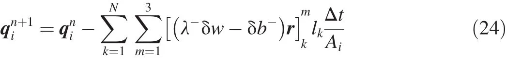
where qniis the vector of conserved variables for cell i at the nth time step;m is the wave number,such that λ-mis the speed of the ingoing m-wave,rmis the right eigenvector corresponding to the m-wave,and δwmand δb-mdenote the mwave components of δw and δb-,respectively;k means the cell edge k,such that lkis the length of the cell edge k;and Aiis the area of cell i.δw is the variation of the wave strength vector w across the cell edge,which can be calculated as follows:

where δq is the variation of q across the cell edge,and R-1is the inverse matrix of R that is composed of the right eigenvectors as column vectors.δb-denotes the ingoing contribution of the source term,with δb being the variation of the source term strength vector across the cell edge,which is calculated as follows:

where δs denotes the variation of the source term across the cell edge.Eq.(24)can be rewritten as follows:

Murillo et al.(2007)show that monotonicity of the conserved variables in the presence of source terms requires the following:

The Courant-Friedrichs-Lewy(CFL)condition restricts the time step of the explicit scheme as follows:

where C is the CFL number,and C ≤ 1;and Δtmaxis calculated as follows:

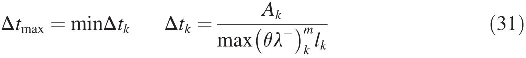
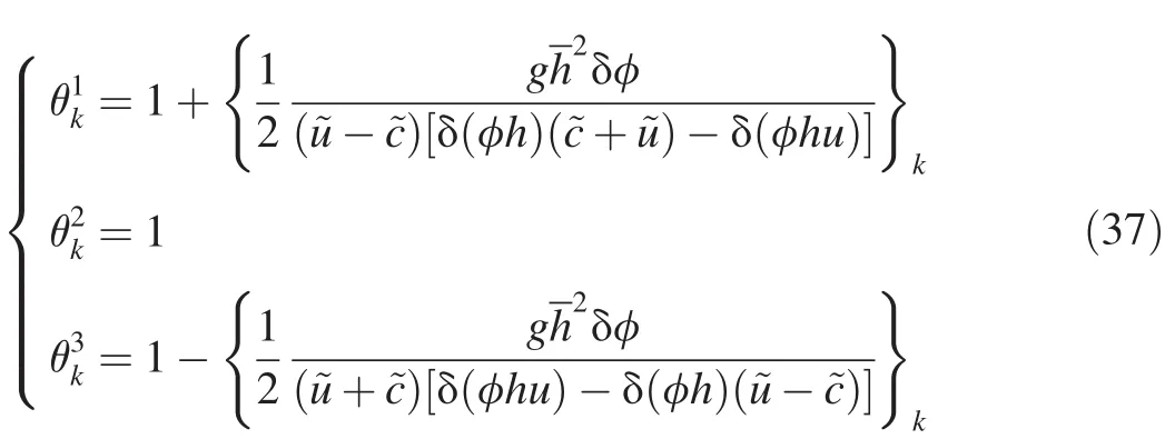
where Akis the minimum of the areas of the cells located at the left and right sides of the cell edge k.For θmk=1,Eq.(31)is identical to the stability condition for homogeneous systems.For 0＜θmk＜1,the stability region of the numerical scheme enlarges,i.e.,larger time steps are allowed,as the source term acts opposite to the flux term.For θmk＜0,the source term dominates theflux term,and the stability region has to be redefined by calculating Δtkas follows:

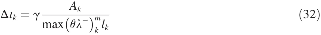
where γ is calculated depending on the constraints of the physical problem,and 0≤γ≤1.

2.3.2.Application of Roe-type solutions to SP model

In the SP model,R and R-1can be calculated as follows:

Using Eq.(25),δw is calculated as follows:

where the tilde denotes that the values are obtained for an intermediate state,e.g.,using Roe-averaged values;δ denotes the variation of a value across the cell edge;and q1,q2,and q3are thefirst,second,and third components of q,respectively.

Using Eq.(26),δb is obtained as follows:

where s2is the second component of the source term s obtained with a suitable numerical discretization.For demonstration purposes,the following discretization is chosen for calculation of δs2:

where h is the average of the water depths at the left and right sides of the cell edge k.Using Eq.(28),can be determined as follows:

2.3.3.Application of Roe-type solutions to AP model

The matrices R and R-1of the AP model are identical to those in Eq.(33).However,because the porosity ψ defined at the cell edge is different from the porosity φ inside the cell in the AP model,variables have to be reconstructed at the edge.Sanders et al.(2008)noted that,for the reconstruction of velocities,φuh and φvh should be used,as they are the conserved variables.The variables are reconstructed forfirst-order accuracy as follows:

The subscript i implies that values are at the center of cell i,and the subscript k implies that values are at the cell edge k.This can be simplified as follows:

It is noted that,because φiis always larger than or equal to ψk,according to Eq.(39),the reconstructed velocities at the edge will always be larger than or equal to the velocities in the cell.The upwind scheme in the wave propagation form is written as

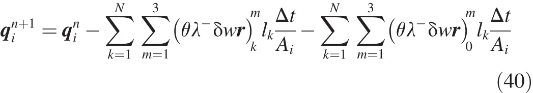
In addition to the waves induced by the variations of theflux vector and source term across the cell edge,additional waves appear due to the differences in theflux vector and source term at the cell center and cell edge,which yield the third term in Eq.(40),described with the subscript 0.Using Eq.(28),θmkand θm0can be calculated,with the major difference being that,in the calculation of θm0,differences between values of δw and δb at the cell center and cell edge are considered,rather than the variations of values across the cell edge.

The monotonicity is ensured when≥ 0.The stability region is defined as the set of time steps satisfying Eq.(30),with C ≤ 1/3,and Δtmaxis calculated as follows:

Then,the stability region enlarges when 0≤θmk≤1 and 0 ≤ θm0≤ 1.For negative values of θmkor θm0,the source term dominates.In Murillo et al.(2007),it is noted that,in this case,the reconstruction of variables should fall back tofirst-order accuracy.However,in the AP model,this is not possible,as the reconstructed results are not the product of a higher-order extrapolation but inherent to the mathematical model.The optimal treatment in these situations has to be addressed in future research.

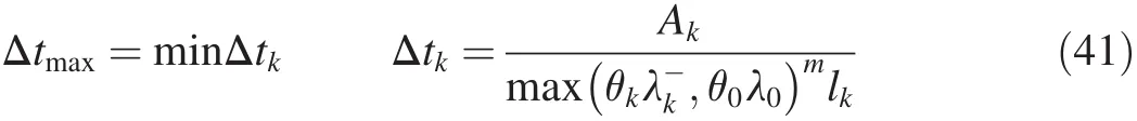
δw and δb are calculated using Eq.(25)and Eq.(26),respectively,as follows:

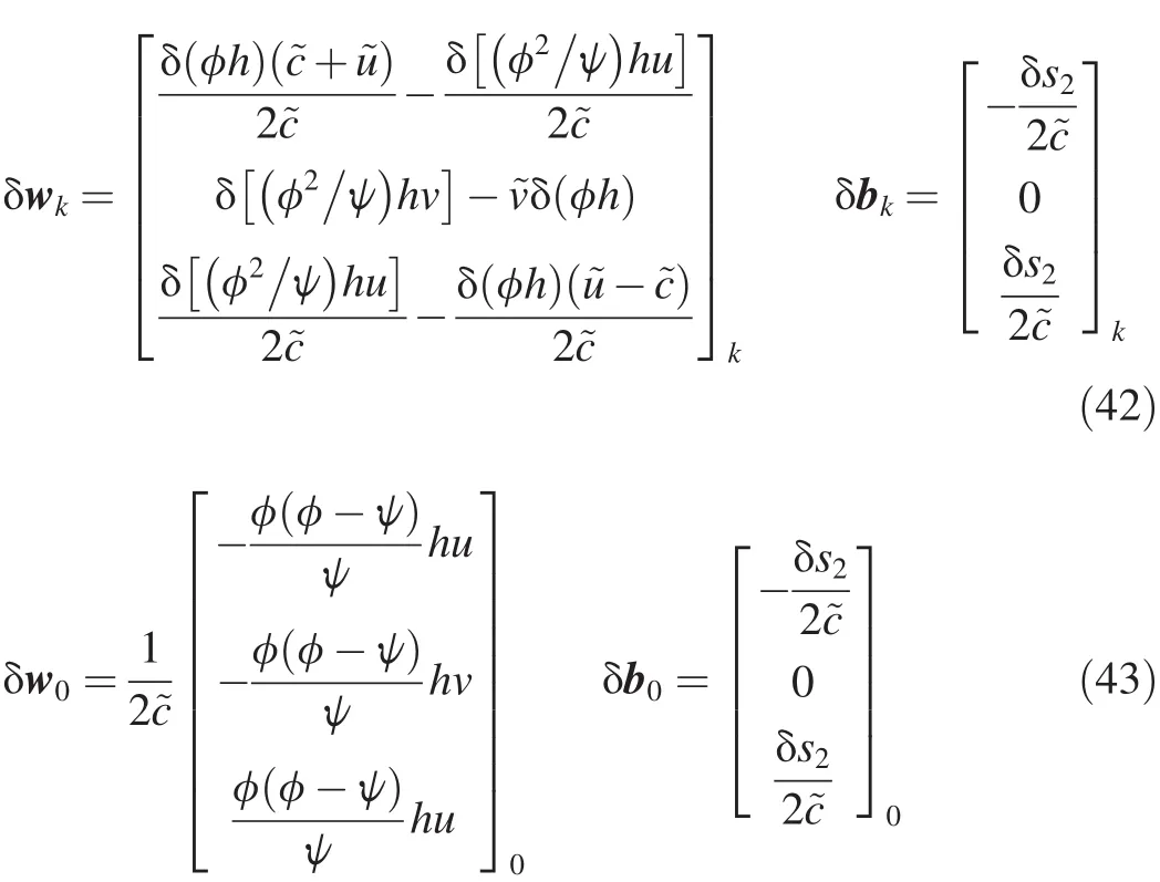
where δs2is calculated as follows:

with hη0to be determined.Then,using Eq.(28),can be determined as follows:

As δs2depends on the slope of hη0,which is constant inside the cell,the second term in the expressions of θ10and θ30in Eq.(46)vanishesinthiscase,withθ10= θ20= θ30.Thisisnottrue when the variation of hη0across the cell edge is considered.

It is worth noting that the ratio φ2/ψ also appears in the momentumflux terms of the porosity shallow water model in Guinot et al.(2017)as well and is a direct result of the assumption that φuh and φvh are conserved between the cell center and edge,i.e.,the continuity is preserved.Guinot et al.(2017)used this relationship to derive an improved version of the AP model,the so-called double integral porosity model.

2.3.4.Discussion

The difference between the SP model and the AP model can be studied by comparing Eq.(37)with Eq.(45)for the same Riemann problem.First,it is assumed that both source term contributions are the same,i.e.,δφ.Direct comparison shows that the only difference is that,in the AP model,δ(uh)is multiplied by the ratio φ2/ψ instead of φ.

Now the source term contributions are not assumed to be equal anymore,and θmkin both models is examined in more detail.Given that,for both models,the right eigenvectors are the same as those in the classical shallow water model,it can be assumed that Roe-averaged values give a sufficient approximation of the middle state for both models(Roe,1981).The conveyance porosity in the AP model is calculated as the minimum of the storage porosity at the left and right sides of the cell edge.Then,θmkcan be evaluated for different porosity configurations.

Three different Riemann problems with different initial states were studied,in which hL,uL,and φLwere the initial water depth,velocity,and porosity,respectively,constituting the left set of initial values,and hR,uR,and φRwere the initial water depth,velocity,and porosity,respectively,constituting the right set of initial values,for the Riemann problem.In case 1,the initial states were defined as hL=10 m,hR=1 m,uL=1 m/s,and uR=0.5 m/s.In case 2,the left-and rightside water depths were switched(velocities remained the same).In case 3,the left-side water depth was set equal to the right-side water depth(velocities remained the same).

Fig.1 shows the evaluation of θ1k,where the region with 0≤ θ1k≤ 1 is colored grey and referred to as the stabilityenhancing region.The evaluation of the SP model is shown in Fig.1(a),(b),and(c),where φL= φRmeans that θ1k=1.It is seen that the stability-enhancing region is mirrored over the line φL= φRin case 1 and case 2(Fig.1(a)and(b)).The largest stability-enhancing region is obtained with equal water depths(Fig.1(c)).In this case,if the values of φLand φRare close to each other with φL＞ φR, θ1kleaves the stability-enhancing region.The stability-reducing region is not symmetric due to the initial velocities.

Fig.1.θ1kfor different porosity and water depth configurations in different cases for SP model and AP model.

Fig.1(d),(e),and(f)show the evaluation of θ1kfor the AP model.It is seen that the stability-enhancing region is more sensitive to water depths.This is because the source term is directly related to the water depth variation across the cell edge(Eq.(44)).Consequently,if hL=hR,the stabilityenhancing region comprises all porosity configurations,as the source term vanishes;if the water depths are not equal,the size of the stability-enhancing region is reduced significantly,compared with the SP model.Very similar observations can be made forFor sake of brevity,this discussion is omitted here.

Issues related to the maximum allowable time step are more complicated.The CFL number C for the AP model is not allowed to exceed 1/3,while C for the SP model is allowed to take values up to 1.In addition,due to the required reconstruction of variables in the AP model,additional waves emerge and must be taken into consideration when the time step is calculated(Eq.(41)).It might be concluded that the time steps of the AP model are more severely restricted.However,at the same time,the wave propagation speeds of the AP model are always smaller than those of the SP model,comparing Eq.(23)to Eq.(11).

Neglecting the source terms,Sanders et al.(2008)provided a stability condition for the AP model based on the homogeneous system as follows:

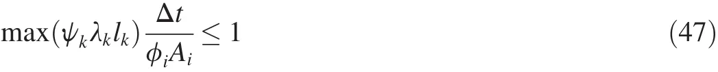
while Guinot and Soares-Fraz~ao(2006)showed that for the homogeneous system the stability condition of the SP model is

which leads to the same conclusions,i.e.,as the wave propagation speeds of the AP model decrease,larger time steps might be allowed.In the authors'experience,the time step of the AP model tends to be smaller compared to that of the SP model in most cases.

3.Computational test cases

Both equations were solved using afirst-order Godunovtypefinite volume scheme with explicit time integration.The numerical scheme of the SP model was presented in Guinot and Soares-Fraz~ao(2006)and is a so-called lateralized scheme,where the influence of the source terms was considered a correction term to the numericalflux.A specialized porous Harten,Lax,and van Leer(HLL)approximate Riemann solver was used for the numericalflux calculation.

The numerical scheme of the AP model calculated the numerical flux through an HLL solver with simplified wave speed estimates.The discretization of the source terms with the C-property preserved,presented in¨Ozgen et al.(2016a),was used.

3.1.One-dimensional dam break with variable porosity

This test case was initially presented in Guinot and Soares-Fraz~ao(2006)and featured a one-dimensional dam break in a domain with variable porosity.The domain was 100 m long and the dam was placed at x=50 m.At the left side of the dam(x ＜ 50 m),an initial water depth of 10 m was defined,and at the right side(x＞50 m),an initial water depth of 1 m was defined.The porosity increased linearly from 0 at x=0 to 1 at x=100 m.The domain was discretized,with a cell size of 0.1 m,and results are plotted for t=4 s.A reference solution was calculated by solving a circular dam-break problem with a radius of 50 m and initial water depths of 10 m inside the dam and 1 m outside the dam(Guinot and Soares-Fraz~ao,2006).

In this test case,the porosity varied smoothly and the cell size was sufficiently small.Therefore,the conveyance porosity in the AP model was always very close to the storage porosity(ψ/φ≈1),and the gradient of the porosity in the SP model was negligible.Thus,it is expected that both models behave similarly.Results for water depth andflow velocity are plotted in Fig.2(a)and(b),respectively,and indeed it can be seen that the models converge to the reference solution in a very similar manner.

3.2.One-dimensional stationaryflow with rapidly varying porosity

Initially presented in Sanders et al.(2008),this test case considered stationaryflow in a one-dimensional channel in the face of a sudden porosity variation.The domain was 1000 m long and the porosity was defined as follows:φ =1 for x ＜400 m and x＞600 m,φ=0.75 for x＞410 m and x＜590 m,φ decreased linearly from 1 to 0.75 between x=400 m and 410 m,and φ increased linearly from 0.75 to 1 between x=590 m and 600 m.The porosity function is plotted in Fig.3.The domain was discretized,with a cell size of 0.25 m,and the model was run until a steady state was reached.A reference solution was obtained by solving the equivalent problem of a narrowing channel based on energy conservation(Bernoulli's law).

Results for water depth andflow velocity are plotted in Fig.4(a)and(b),respectively.Both models behave similarly and converge to the steady-state solution,because,again,the variation of the porosity was smooth.Moreover,in the AP model,the conveyance porosity was close to the storage porosity,i.e.,ψ/φ≈1,and the gradient of the porosity in the SP model was negligible.

3.3.One-dimensionaldambreakwithporositydiscontinuity

This test case was initially presented in Guinot and Soares-Fraz~ao(2006)and comprised a dam break with porosity discontinuity.The domain was 100 m long,with the dam positioned at x=50 m,separating an initial water depth of 10 m and a porosity of 1 at the left side and an initial water depth of 1 m and a porosity of 0.1 at the right side of the dam.The domain was discretized,with the size of cells of 0.01 m.A reference solution was calculated by solving the Riemann problem with porosity suggested in Guinot and Soares-Fraz~ao(2006),which yielded a nonlinear system of seven equations for seven unknowns that could be solved iteratively using,e.g.,the Newton-Raphson procedure.The reference solution was thus based on the mathematical model of the SP model.

In this test case,the variation in the porosity had a sudden discontinuity.In the AP model,at the position of the discontinuity,the conveyance and storage porosities differed from each other significantly.In the SP model,the gradient of the porosity yielded a significant source term.Thus,a deviation in model results is expected.In Fig.5,where model results are plotted against the reference solution at t=4 s,it is observed that the results of the models deviate from each other.The results of the SP model are closer to the reference solution,while those of the AP model clearly deviate from it.Comparison with the reference solution shows that the shock position is inconsistent with theAPmodel,andthevelocityandwaterdepthoftheAPmodel are overestimated downstream of the dam.

Here,it is noted that the AP model does not account for a porosity discontinuity across the cell edge in its mathematical model.The deviation in the results is therefore also due to a structural deviation between both models.

Fig.2.Results of one-dimensional dam break of AP model and SP model with variable porosity at t=4 s.

Fig.3.Stationaryflow with rapidly varying porosity in onedimensional channel.

3.4.Discussion

The numerical test cases support thefindings in Section 2,that in cases where the conveyance porosity differs signifi-cantly from the storage porosity,the AP model behaves differently from the SP model,and in cases where the conveyance porosity is close to the storage porosity,both models behave similarly.

In order to study this deviation in more detail,we consider the cell(without loss of generality)at the discontinuity(x=50.05 m)in Section 3.3.At t=0,at the cell edge located at the dam position,the following Riemann problem is solved with the SP model and the AP model,with the initial conditions as follows:hL=10 m,hR=1 m,φL=1,φR=0.1(ψ =0.1),and φLqL= φRqR=1 m2/s,where qLand qRare the unit-width discharges at the left and right sides of the cell edge,respectively.Calculating velocities at the cell edge,which will be the input of the Riemann solver forflux calculation,gives the following results of the SP model:

and the following results of the AP model:

which means that for different values of the conveyance porosity and storage porosity,differentflow velocities are reconstructed at the cell edge,which in turn means that different Riemann problems are solved.Note that only the reconstructed velocities of the AP model and the BP model differ from each other,and the water depth at the cell center is used as the cell edge value in the AP model(Eq.(38))as well as in the SP model.

It is easy to show that if the conveyance porosity equals the storage porosity,the AP model and SP model solve the same Riemann problem.Consider the Riemann problem with the following initial conditions:hL=10 m,hR=1 m,φL=0.1,φR=0.1(ψ =0.1),and φLqL= φRqR=1 m2/s.Now,reconstructed velocities used in the Riemann solver yield the same results of the SP and AP model:uL=1 m/s and uR=10 m/s.Thus,both models solve the same Riemann problem in this case.

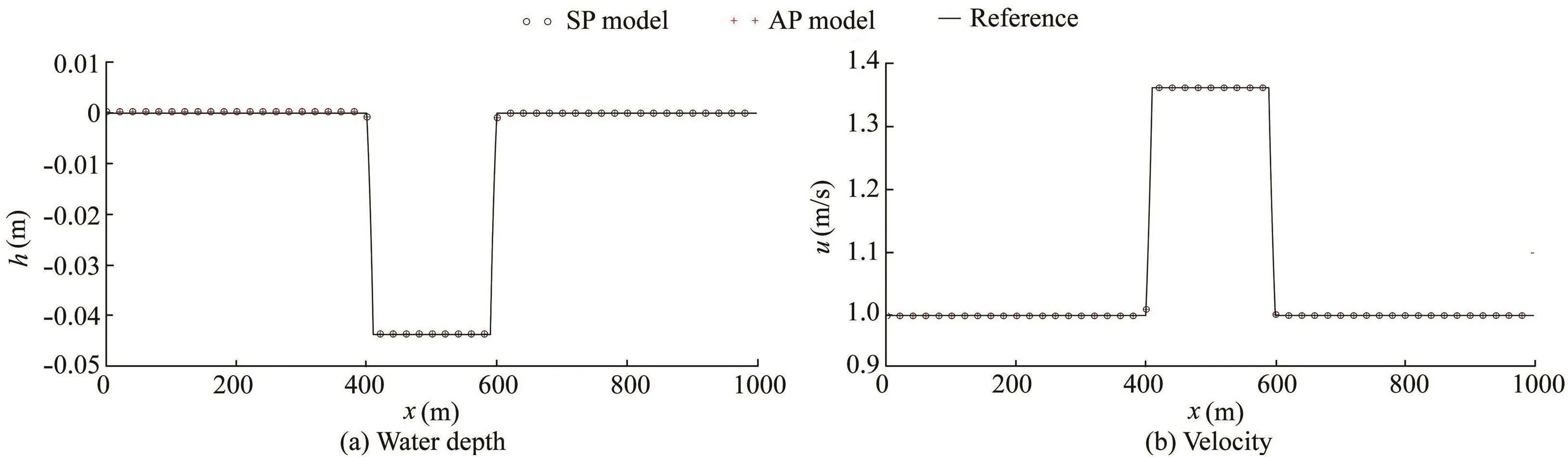
Fig.4.Steady-state solutions of AP model and SP model with rapidly varying porosity.

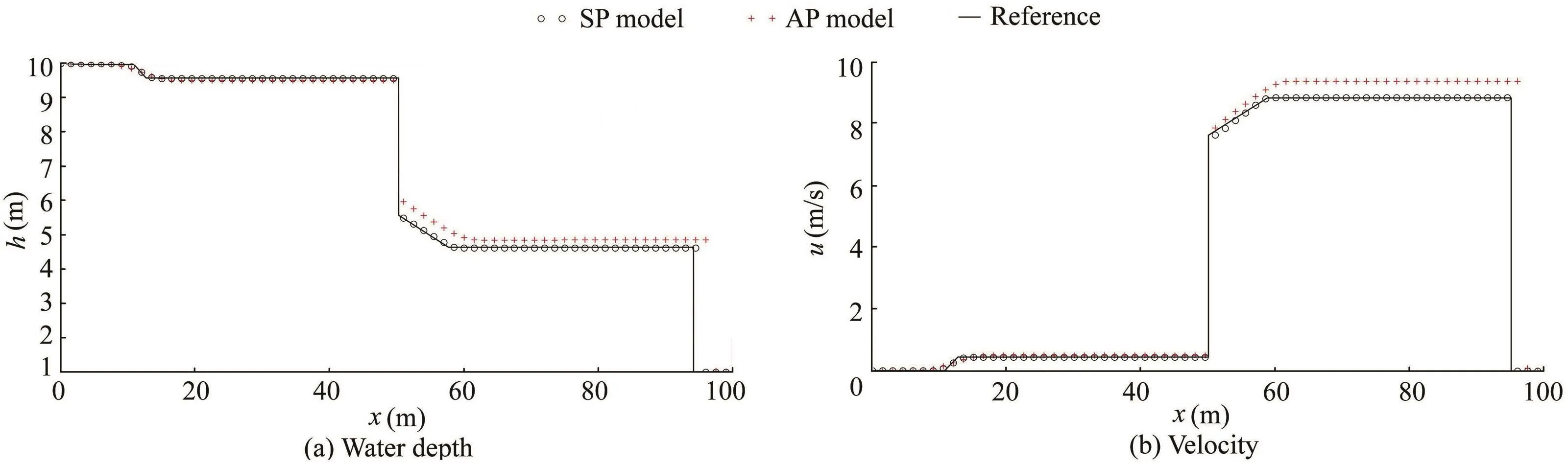
Fig.5.Results of one-dimensional dam break of AP model and SP model with porosity discontinuity at t=4 s.

In addition,in cases with a sudden porosity discontinuity,the geometric source term of the SP model becomes signifi-cant and enhances the SP model results,while the AP model does not account for this process.

3.5.Two-dimensionaldam-breakflowthroughidealizedcity

Both models were used to replicate a laboratory experiment conducted at the Universit′e Catholique de Louvain,Belgium(Soares-Fraz~ao and Zech,2008).The computational domain is shown in Fig.6.In the reservoir on the left side,an initial water level elevation of 0.40 m was defined.On the right side of the reservoir,an initial water level elevation of 0.011 m was set.A simplified building block was placed in the domain as sketched in Fig.6,where individual houses are colored grey.The gate between both areas was opened at t=0,inducing a dam-breakflow.Measurement data for the water level elevation were available from gauges placed between and in front of the houses.The locations of some gauges used in the following analysis are shown in Fig.7.The total simulation time was 15 s.Both models took about the same time to run the simulation with an average time step of 0.02 s.

Both the AP model and the SP model used structured meshes with a cell size of 0.25 m.The friction was accounted for by means of a Manning's coefficient of n=0.01 s/m1/3.In addition,a simple drag force closure was applied in both models,using a building drag coefficient of cbD=5 m-2.The storage porosity of the cells was deduced directly from the underlying buildings,i.e.,the fraction of the cell occupied by a building was calculated individually in each cell.For the AP model,the conveyance porosity was calculated in the same way.No further calibration was carried out.

Fig.6.Top view of computational domain with initial conditions(units:m).

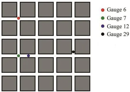
Fig.7.Locations of some gauges.

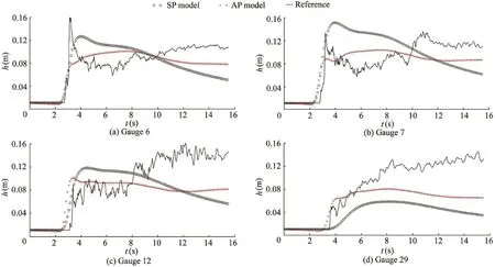
Fig.8.Comparison of computed and measured water level elevations at different gauges.

Results at different gauges are compared in Fig.8.In the two-dimensional test case,the models diverge significantly from one another.It is observed that the AP model shows better agreement with measured data than the SP model.In the twodimensional case,several factors lead to the difference in the model results.First,in cases with more complex geometry,the additional conveyance porosity of the AP model significantly enhances model results.The blocking and diversion of water duetothebuildingscanberepresentedmoreaccuratelywiththe addition porosity term.The large difference between results of the AP model and the SP model at gauge 29 can be explained as follows:whenwaterarrivesatthisgauge,ithasalready traveled through almost the entire porous medium representing the building block,and water is not being blocked sufficiently at this gauge in the SP model.However,more water is diverted in the AP model due to its additional porosity term at the cell edges,causing large deviations between both model results.In addition,at the gauges located more toward the front,i.e.,gauges 6,7,and 12,it is observed that the models show greater agreementatthebeginningofthesimulationbutdivergeastime passes,with the SP model consistently showing more deviation from the measured data than the AP model.

The second reason for the deviation is related to the cell size of the computational mesh.In Soares-Fraz~ao et al.(2008)and Velickovic et al.(2017),the resolution of the SP model was not designed to be as coarse as it was in this test case.For example,in Velickovic et al.(2017)the cell size was smaller than the building scale,and the porosity terms were usually used to further calibrate the model instead of using the layout of the building array to calculate the porosity terms(Soares-Fraz~ao et al.,2008).Because neither of these strategies was used in the present case,the accuracy of the SP model was diminished.It can be concluded that,if the porosities are calculated based on the topography at the sub-grid scale,the AP model should be preferable.

4.Conclusions

A comparison between the SP model(Guinot and Soares-Fraz~ao,2006)and the AP model(Sanders et al.,2008)was presented.

The influence of the source term was analyzed using Roetype approximate solutions that were initially presented in Murillo et al.(2007).It is seen that the ratio ψ/φ significantly influences the model behavior.If the ratio is close to 1,which implies smooth variation of porosity,similar behavior can be expected of both models,because the wave propagation speeds are similar and the geometric source term of the porosity gradient in the SP model is negligible.In addition,the analysis shows that the different source terms of the models yield different behaviors,depending on the configurations of porosities and water depths.

Computational test cases were carried out to further study the influence of the ratio ψ/φ on model results.Computational results support the conclusions of theoretical analysis.In cases with smooth porosity variation,the different model results converge toward each other while,in the face of sudden porosity changes,model results deviate.

It is emphasized that the deviation of the results of the AP model from the reference solution in the case of a onedimensional dam break with porosity discontinuity does not have implications for the model quality.The reference solution has been derived by solving the Riemann problem for the SP model and it is therefore reasonable that the results of the SP model show better agreement with the reference solution in this test case.

The source terms in each model behave differently.The porosity gradient source term in the SP model accounts for spatial variations in porosity that drive water from regions with low porosity to regions with high porosity.Consequently,the influence of the source term is strong if the difference in porosities at both sides of the cell edge is large.In contrast,the source term in the AP model accounts for a pressure exchange at the interface between water and buildings,and it is not influenced by the difference in porosities at both sides of the cell edge.In the AP model a conveyance porosity is defined at the edge,i.e.,the AP model has no mechanism to account for a porosity discontinuity.The source term in the AP model depends only on the water depth configuration at the edge.

A two-dimensional test case was presented to compare both models in a more complex setting.Model results significantly deviate from each other.The AP model shows better agreement with measured data.The conveyance porosity,which is absent from the SP model,significantly enhances the results of the AP model.It can be concluded that,if the porosities are calculated based on the topography at the sub-grid scale,the AP model is preferable.

Bird,R.B.,Stewart,W.E.,Lightfood,E.N.,2007.Transport Phenomena,second ed.John Wiley&Sons,New York.

Cunge,J.A.,Holly,F.M.,Verwey,A.,1980.Practical Aspects of Computational River Hydraulics.Pitman Advanced Publishing Program,London.

Defina,A.,2000.Two-dimensional shallow flow equations for partially dry areas.Water Resour.Res.36(11),3251-3264.https://doi.org/10.1029/2000WR900167.

Ferrari,A.,Vacondio,R.,Dazzi,S.,Mignosa,P.,2017.A 1D-2D shallow water equations solver for discontinuous porosityfield based on a generalized Riemann problem.Adv.Water Resour.107,233-249.https://doi.org/10.1016/j.advwatres.2017.06.023.

Guinot,V.,Soares-Fraz~ao,S.,2006.Flux and source term discretization in two-dimensional shallow water models with porosity on unstructured grids.Int.J.Numer.Meth.Fluid.50(3),309-345.https://doi.org/10.1002/fld.1059.

Guinot,V.,2012.Multiple porosity shallow water models for macroscopic modelling of urbanfloods.Adv.Water Resour.37,40-72.https://doi.org/10.1016/j.advwatres.2011.11.002.

Guinot,V.,Sanders,B.F.,Schubert,J.E.,2017.Dual integral porosity shallow water model for urbanflood modelling.Adv.Water Resour.103,16-31.https://doi.org/10.1016/j.advwatres.2017.02.009.

Hinkelmann,R.,2005.Efficient Numerical Methods and Informationprocessing Techniques for Modeling Hydro-and Environmental Systems.Springer-Verlag,Berlin.

LeVeque,R.J.,2002.Finite Volume Methods for Hyperbolic Problems.Cambridge University Press, New York. https://doi.org/10.1017/CBO9780511791253.

Mohamed,K.,2014.Afinite volume method for numerical simulation of shallow water models with porosity.Comput.Fluid 104,9-19.https://doi.org/10.1016/j.compfluid.2014.07.020.

Murillo,J.,García-Navarro,P.,Burguete,J.,Brufau,P.,2007.The influence of source terms on stability,accuracy and conservation in two-dimensional shallow flow simulation using triangularfinite volumes.Int.J.Numer.Meth.Fluid.54(5),543-590.https://doi.org/10.1002/fld.1417.

Nepf,H.,1999.Drag,turbulence,and diffusion inflow through emergent vegetation.Water Resour.Res.35(2),479-489.https://doi.org/10.1029/1998WR900069.

¨Ozgen,I.,Liang,D.,Hinkelmann,R.,2016a.Shallow water equations with depth-dependent anisotropic porosity for subgrid-scale topography.Appl.Math. Model. 40(17-18), 7447-7473. https://doi.org/10.1016/j.apm.2015.12.012.

¨Ozgen,I.,Zhao,J.,Liang,D.,Hinkelmann,R.,2016b.Urbanflood modeling using shallow water equations with depth-dependent anisotropic porosity.J.Hydrol.541,1165-1184.https://doi.org/10.1016/j.jhydrol.2016.08.025.

Roe,P.L.,1981.Approximate Riemann solver,parameter vectors,and difference schemes.J.Comput.Phys.43(2),357-372.https://doi.org/10.1016/0021-9991(81)90128-5.

Sanders,B.F.,Schubert,J.E.,Gallegos,H.A.,2008.Integral formulation of shallow-water equations with anisotropic porosity for urban flood modeling. J. Hydrol. 362(1-2), 19-38. https://doi.org/10.1016/j.jhydrol.2008.08.009.

Schubert,J.E.,Sanders,B.F.,2012.Building treatments for urbanflood inundation models and implications for predictive skill and modeling efficiency.Adv.Water Resour.41,49-64.https://doi.org/10.1016/j.advwatres.2012.02.012.

Soares-Fraz~ao,S.,Lhomme,J.,Guinot,V.,Zech,Y.,2008.Two-dimensional shallow-water model with porosity for urbanflood modelling.J.Hydraul.Res.46(1),45-64.https://doi.org/10.1080/00221686.2008.9521842.

Soares-Fraz~ao,S.,Zech,Y.,2008.Dam-breakflow through an idealised city.J.Hydraul.Res.46(5),648-658.https://doi.org/10.3826/jhr.2008.3164.

Velickovic,M.,Zech,Y.,Soares-Fraz~ao,S.,2017.Steady-flow experiments in urban areas and anisotropic porosity model.J.Hydraul.Res.55(1),85-100.https://doi.org/10.1080/00221686.2016.1238013.