An efficient dynamic uniform Cartesian grid system for inundation modeling

Jing-ming Hou,Run Wng,Hi-xio Jing,*,Xi Zhng,Qiu-hu Ling,Yn-yn Di

aInstitute of Water Resources and Hydro-Electric Engineering,Xi'an University of Technology,Xi'an 710048,China bSchool of Civil Engineering and Geosciences,Newcastle University,Newcastle Upon Tyne NE1 7RU,UK

cHydrology Bureau,Yellow River Conservancy Commission,Zhengzhou 450004,China

1.Introduction

Flooding is a type of natural disaster that raises an enormous threat to lives and property.This threat is likely to escalate as a result of global warming and climate change.For example,southern England has seen the wettest winter for more than 200 years from 2013 to 2014,leading to severe and long-lastingflooding in Somerset.According to data provided by the Flood Protection Association(FPA)in the UK,of the 28 million homes in the UK,over 5 million are currently at risk,as well as over 300000 business premises and many more public and utility services buildings.Moreover,flooding is likely to cause other environmental problems.For instance,it is linked closely to water quality(Hrdinka et al.,2012).Flood prediction,which can be achieved using numerical models,can help guide people toward protection measures for the upcoming floods so that the damage can be significantly alleviated.In recent years,Godunov-typefinite volume schemes have gained more attention inflood simulation,for example in Delis et al.(2008),Liang(2010),Jeong et al.(2012),Hou et al.(2013b),Ata et al.(2013),and Guan et al.(2014),as they are capable of capturing shocks,and preserving accuracy and robustness.

Simulation results have also been proven to be very sensitive to grid resolution(Wilson and Atkinson,2003;Ozdemir et al.,2013).Withfiner grids,more realistic terrain features can be reflected.However,high-resolution modeling of realworldflooding may sometimes require millions of computational nodes or cells to accurately represent the domain topography of afloodplain,making such simulations computationally prohibitive on most existing computers.This signalsa need to make computations faster.There are several approaches to improving the computational efficiency of a flood model.Liu and Pender(2013)used a cellular automata-based rapidflood spreading model to generate an estimated inundation map.Despite the fast computation,this approach fails to computeflow velocities.Another approach solves the simplified governing equations derived by neglecting the dynamic terms in the two-dimensional(2D)shallow water equations(SWEs)(Bates et al.,2010;Wang et al.,2011a).However,the neglected dynamic terms can affect the accuracy of the evaluated velocities,especially forflows with transientflow features.Some researchers have adopted adaptive grids to improve the computation efficiency,for instance George and Leveque(2008),Popinet(2011,2012),and Liang(2012).As mentioned in Liang and Borthwick(2009)and Popinet(2011),when estimating the new values in newly created cells on adaptive grids,of the equations of mass conservation and water surface continuity,only one of the two can be satisfied.Both of these equations are important inflood simulation,as a violation of the former will lead to erroneous inundation areas and unsatisfactory values of the latter will bring about disturbance of the conservation property (C-property)(Bermudez and Vazquez,1994).Due to this deficiency of the adaptive grids,uniform grid-based shallow waterflow models are preferred and attract more attention(Hervouet,2000;Sanders et al.,2010;Pu et al.,2012;Smith and Liang,2013;Xia et al.,2017).As a uniform grid is easy to generate from the produced terrain DEM,the numerical methods can be straightforwardly implemented,and the complex terrain features can be simply reflected by using uniform grids.

To simulate flooding efficiently and accurately,this study used a robust full shallow water model on a dynamic uniform Cartesian grid system,which might optimize the computational grid according toflow features.The governing equations and the numerical scheme for the inundation model are briefly introduced in Section 2;the new grid system is addressed in Section 3 and its performance is demonstrated and analyzed through discussion of a field-scale test case involving flood routing in Section 4 and Section 5;and Section 6 describes thefindings of this study.

2.Governing equations and numerical methods

The numerical inundation model was developed by solving the 2D SWEs numerically,within a framework of a wellbalanced cell-center Godunov-typefinite volume method.The 2D pre-balanced SWEs proposed in Liang and Borthwick(2009)were chosen as governing equations:

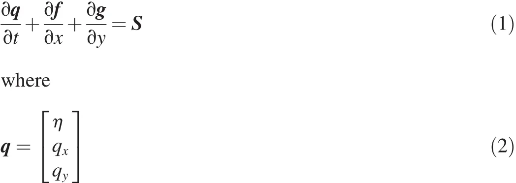
where t is time;x and y are the Cartesian coordinates;q is the vector of conserved flow variables containing η,qx,and qy,which are the free surface water level and the unit-width discharges in the x-and y-directions,respectively;qx=uh and qy=vh;h,u,and v are the water depth and the depthaveraged velocities in the x-and y-directions,respectively;zbis the bed elevation and zb=η-h;f and g are theflux vectors in the x-and y-directions,respectively;S is the source vector;mwis the source or sink of mass caused by rainfall or infiltration;and Cfis the bed roughness coefficient,determined herein as gn2/h1/3,with n being the Manning coefficient.

The SWEs are solved numerically with the two-step MUSCL-Hancock scheme developed in Leer(1984)and adjusted for the SWE simulation in Zhou et al.(2002),within the framework of the Godunov-type cell-centeredfinite volume method for Cartesian grids in Liang(2010,2011,2012),and Smith and Liang(2013).It consists of a predictor step and a corrector step.In the first step,the intermediateflow variables are computed over half of a time interval.Those predicted variables are then utilized in the corrector step to update the results to a new time level.The friction source terms are not evaluated within the MUSCL-Hancock scheme but independently evaluated by a splitting point-implicit method proposed in Liang and Marche(2009).Since the MUSCLHancock isan overallexplicitscheme,the Courant-Friedrichs-Lewy(CFL)condition must be satisfied to ensure solution stability.The CFL condition proposed in Liang(2012)is employed to estimate the time step.Open and closed boundaries are treated as in Liang and Borthwick(2009).In this work,the aforementioned numerical methods are not documented in detail and readers can look them up in the references listed above.

3.Dynamic uniform Cartesian grid system

In practical application,the small-scale features(i.e.,walls and ditches)can have a significant impact on flood propagation.Despite the increased accuracy created by applying a high-resolution grid,it significantly increases of the computational power required to simulateflood events over large domains.For example,Bates(2012)claimed that simulations at very high resolutions(grid resolution of 10 cm)would take 104 times longer than at 2 m.As mentioned in the introduction,there are a couple of means to promoting the efficiency of computation.It was achieved in this study by using a new uniform Cartesian grid system,which can reduce the number of cells under consideration.

Inflood routing,generally speaking,just a small part of the domain is wet initially and the wet part then starts to spread as the river level escalates or the dam or defense breaks,which is actually a problem involving moving wetdry boundaries(Bates and Hervouet,1999).Moving wet-dry boundaries are preferred for computation onfixed grids,as shown in Liang and Marche(2009),Delis and Nikolos(2013),and Hou et al.(2013c),asfixed grids are easy to generate and can avoid the numerical difficulties induced by dynamically adaptive grids.However,fixed grids will lead to massive amounts of redundant dry cells,which take up a large amount of memory and computational effort in inundation simulation.While the schemes proposed,for example,by Wang et al.(2011b)and Hou et al.(2013a)can avoid the computation offlow variables on dry cells away from wet-dry interfaces(white cells sketched in Fig.1),a loop to identify these cells is still required.Moreover,these dry cells may become wet later in the computation and must be stored in the memory throughout the simulation.However,certain cells remain dry at all times,and thus are not necessarily required in the simulation.As the inundation area is unknown before simulation,it is impossible to determine the location of persistently dry cells.To avoid underestimation of theflooded area,a computational domain that covers a lot of persistently dry cells is commonly used(Fig.1),for example the rectangular domains used in Liang(2010)and Singh et al.(2011).Apparently,simulation efficiency can be improved by removing the persistently dry cells.Based on the idea described above,a new uniform Cartesian grid system was developed to discard persistently dry cells in inundation simulation(Fig.2).

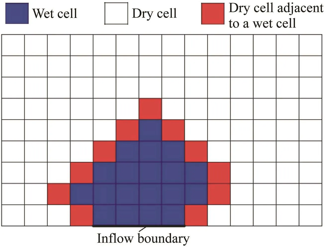
Fig.1.Conventional uniform Cartesian grid forflood simulation.

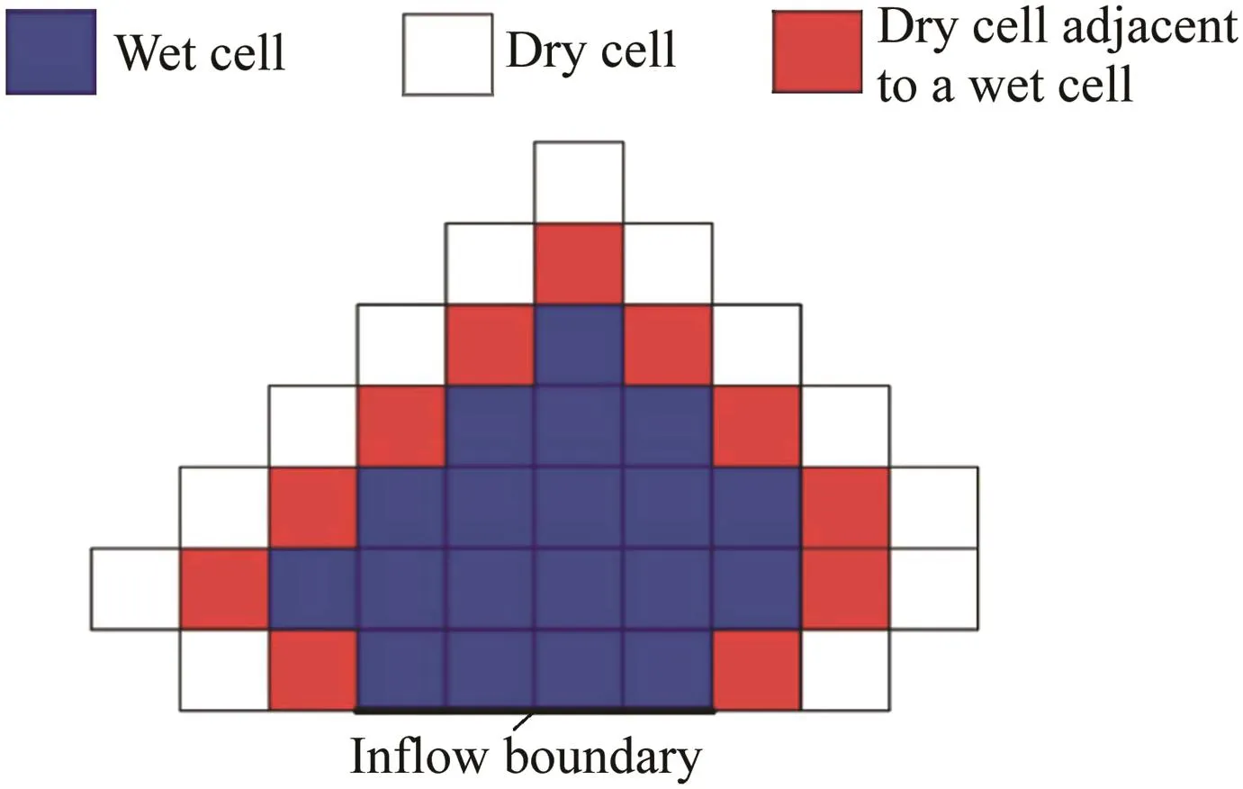
Fig.2.New uniform Cartesian grid forflood simulation.

The new grid system was created according toflood features.When theflood spreads,the grid expands dynamically to cover wet cells and two layers of dry cells adjacent to wet cells(in this study,wet and dry cells were determined by checking if the water depth was higher than a criterion of 10-6m).In contrast,the grid remains static when theflood recedes;the reason for this is addressed in the last paragraph of this section.That means new wet cells are added to the grid system in wetting,but no cells are deleted in drying.In a time step,the new uniform Cartesian grid is generated following the steps below:

Step 1:Dry cells are identified adjacent to wet ones.These dry cells are termed root cells in this paper and are actually the boundary cells of an inundation area.If it is thefirst time step,the root cells are defined from the initial and boundary conditions.They can be the dry cells next to water bodies,inflow boundaries,dikes,or dam breaches,from which water will burst into the area under consideration.For example,root cells with ID numbers of 1,2,3,and 4 were generated near an inflow boundary in this study,as illustrated in Fig.3(a).

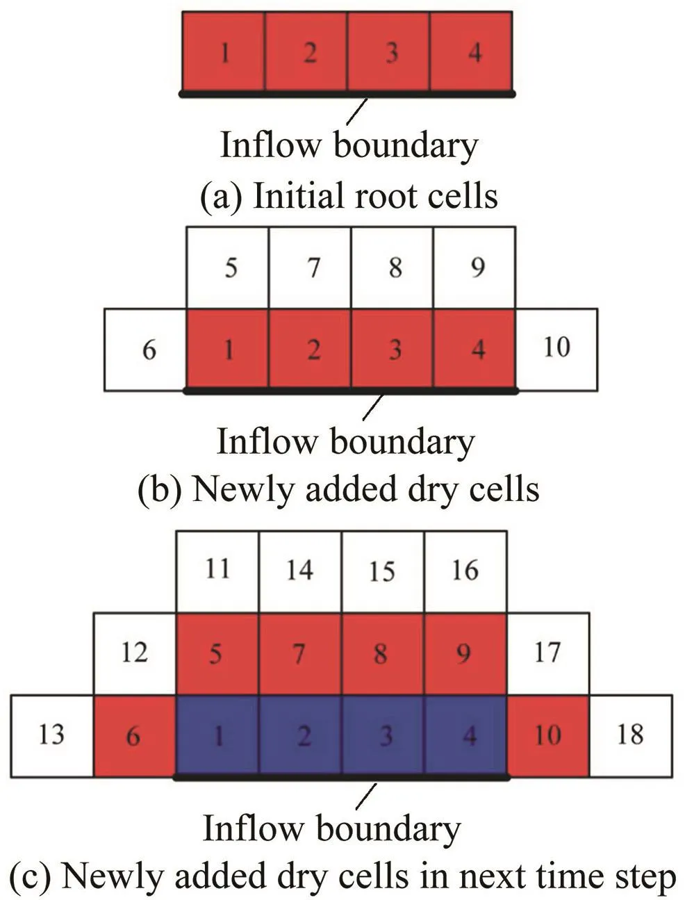
Fig.3.New uniform Cartesian grid generation.

Step 2:A layer of dry cells is extended from the root cells identified in last step.The extension is carried out cell by cell.For instance,if root cell 1 is under consideration,four substeps are required to add new dry cells:(1)A loop over all four neighboring cells is taken to check whether a neighboring cell has already been added to the grid.(2)If the above condition is not satisfied for a neighboring cell,a new cell is added to the grid.For example,as cell 1 does not have northern and western neighboring cells,new dry cells 5 and 6 are added,respectively,as plotted in Fig.3(b).(3)The bed elevation and theflow conditions of zero water depth and velocities are imposed on the newly created dry cells.(4)The neighboring information of the newly added dry cells is determined.If there are no neighboring cells,the neighboring cell ID is specified as 0.Meanwhile,the neighboring information of root cells should be updated for future use.For example,the neighboring cell IDs for root cell 1 are 5,2,-1,and 6 to the north,east,south,and west,respectively(Fig.3(b)).A negative ID signifies an inflow boundary.

Step 3:After a layer of dry cells is added,the aforementioned Godunov-typefinite volume scheme is employed to compute the values offlow variables at the new time level for all cells excluding the newly added dry cells.As the newly added dry cells are next to dry cells,it must be dry cells at the new time level when using the explicit method(it is out of the question to obtain netfluxes of mass).For example,we only computed thefluxes and source terms for cells 1 through 4 in Fig.3(b).In fact,the newly added dry cells are just used to computefluxes and source terms of the roots cells.The updatedflow variables indicate that cells 1 through 4 turn out to be wet at the new time level.Therefore,as illustrated in Fig.3(c),the cells 1 through 4 are wet grids depicted in blue.The red and white grids both are dry cells,but the white grids,i.e.the newly created dry cells,are out of the calculation in this time level.

The procedure from Step 1 to 3 is repeated to generate the grid and compute theflood spreading until the desired time.For instance,in the second cycle,the newly created grid is demonstrated in Fig.3(c).

Noticeably,the new grid is generated through addition of cells,and no subtraction is taken into account,because deleting a cell from a grid will lead to the reconstruction of all cell IDs and in turn the neighboring cell information.Therefore,the improved efficiency through reduction of cell number is likely to be offset by the reconstruction for the cell ID and neighboring information.In addition,flood recession may give rise to discontinuous wet patches,which make the grid too complex.That is why the grid will not shrink in the drying process,i.e.,when theflood starts to subside.It is unhelpful to have some redundant dry cells,which may affect the efficiency in the drying process.However,in comparison to the conventional uniform Cartesian grid system,the redundant dry cells are much fewer in the new grid system and it remains preferable.Unlike the dynamic adaptive grid,the new grid system employs uniform square cells in the dynamic process,no refining and coarsening are demanded in simulation,and the system does not involve the problem of preserving the C-property and mass conservation at the same time.It should be noted that the new grid system will not increase the model's efficiency forflash flood simulation,because the heavy rainfall will wet the entire domain and no redundant dry cells will exist.In this case,the new grid system becomes a regularfixed uniform gird.

4.Simulation of defense-breakflood in Thamesmead

The performance of the Godunov-typefinite volume scheme has beenverified widely,for example in Wang et al.(2011b)and Liang(2010,2011,2012).Inordertoaccentuatetheadvantageof thenewgridsystemintermsofefficiency,afield-scalefloodwas modeledwiththeGodunov-typefinitevolumescheme,includingfloodspreadingandsubsidenceprocesses,onthenewgridaswell asonaconventionaluniformCartesiangrid.Afictionalfloodwas assumedtobecausedbyariverburstingitsbankinThamesmead,England.Grid resolutions of 5 m and 10 m were chosen for both grids and the dimensions of the computational domain for the conventional uniform Cartesian grid were set to be 5000 m×4000 m,as shown in Fig.4.Fig.4 also indicates a 140mlongbreachfromwhichthefloodflowsintothefloodplain.The inflow hydrograph is shown in Fig.5.A constant infiltration rate of 2.5 × 10-5m/s and Manning coefficient of 0.035 s/m1/3were specified across the flood plain.The simulations on both grids were carried out on a desktop computer with an Intel i5-3470 CPU(four cores with a clock speed of 3.2 GHz)and 8G RAM,for 54000 s with a Courant number of 0.5.

5.Results and discussion

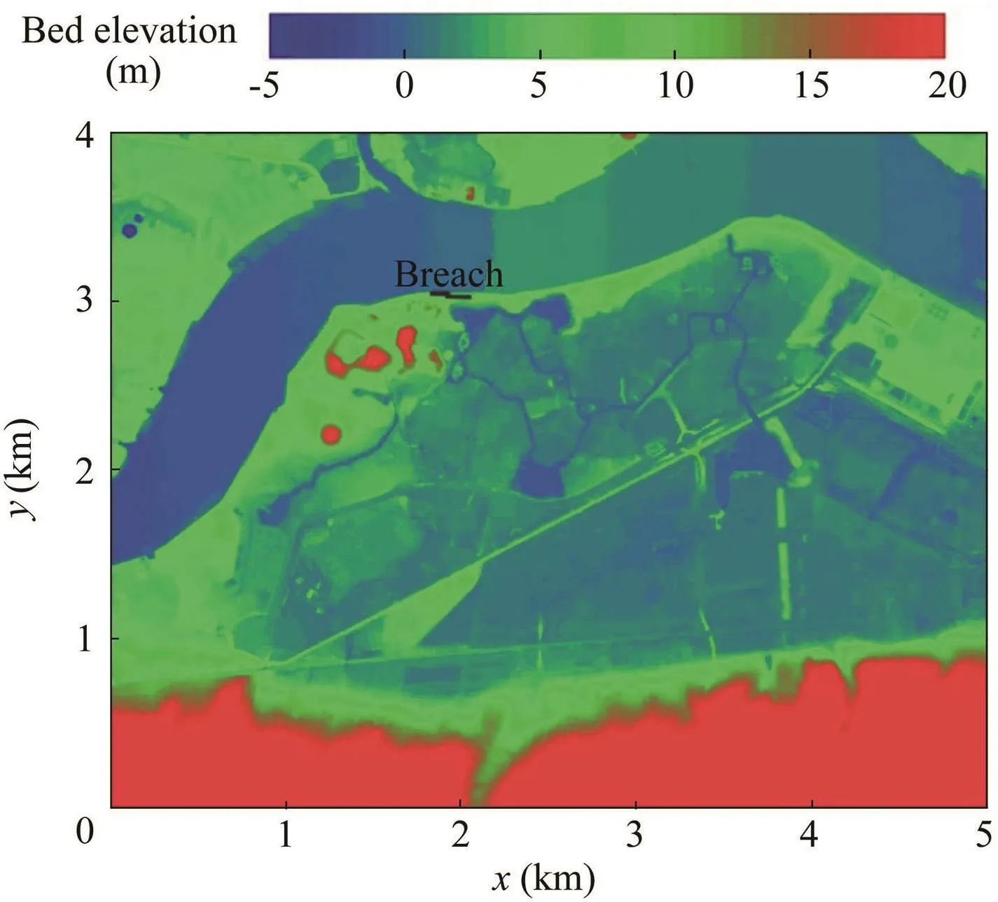
Fig.4.Topography data of Thamesmead.

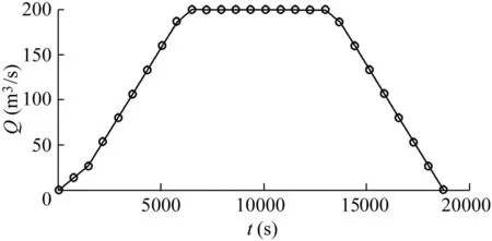
Fig.5.Inflow hydrograph from breach.

Fig.6 compares the computedflood maps in terms of water depth on the new uniform Cartesian grid and the conventional one with 5-m grid resolution at t=2 h,5 h,and 8 h.The results are exactly the same,as the new grids are able to cover all required wet cells and adjacent dry ones.To demonstrate this clearly,three schemes have been examined:the conventional uniform Cartesian grid with 10-m grid resolution(the coarser grid simulation),the conventional uniform Cartesian grid with 5-m grid resolution(thefine grid simulation),and the dynamic uniform Cartesian grid with 5-m grid resolution(the new grid simulation).The computed water level evolutions at three gauges(G1(3185 m,1545 m),G2(3685 m,2075 m),and G3(2805 m,2655 m))are compared in Fig.7 for both grids.The computed water levels on the new grid and thefine one coincide perfectly,which further indicates that the new grid does not affect the accuracy of the modeling.Thus,if the new grid can speed up the simulation forfloods,it will be a promising alternative to the conventional uniform Cartesian grid.In addition,Fig.7 demonstrates that the real-word inundation simulation is quite sensitive to the grid resolution,and thus high resolution is required.

Fig.6.Computedflood map at different situations.

Fig.7.Computed water level at different gauges.

Since the new grid was developed to avoid the dry cells that are not involved in inundation simulation,the grid should evolve in accordance withflood spreading.Fig.8,along with Fig.6,demonstrates theflood spreading and the grid evolution and suggests that the new grid expands along with the wet-dry front moving with the spreadingflood.The time history of the cell number on two grids is plotted in Fig.9.A clear upswing of the total cell number for the new grid is observed inflood spreading,but it remains nearly constant after the maximum inundation takes place around t=8 h(Fig.10).The maximum cell number recorded was 147469.In contrast,the conventional grid has 800000 cells throughout the simulation.A large amount of redundant cells are successfully excluded by the new grid system.However,as the dry cells away from wet cells do not demand the computation offluxes and source terms,the efficiency increase is not directly proportional to the reduced cell number.From the computational time shown in Fig.11,the new grid is far more economical than the conventionalone.Fig.11 quantitatively demonstratesthe improved efficiency of the new grid system.It can save more than 34%of the computational effort(it is 52%faster)even in the flood recession process,when the grid is almostfixed and in turn some dry cells appear.Yet there are many more redundant dry cells on the conventional grid than on the new grid throughout the simulation,as plotted in Fig.12.In a nutshell,the new grid system can greatly improve the computational efficiency by reducing the redundant dry cell number.In the meantime,the accuracy of the scheme is not affected at all.

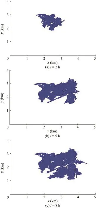
Fig.8.Grid evolution on new grid at different time.

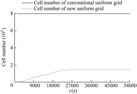
Fig.9.Cell number on two grids.

Fig.10.Flood propagation and grid evolution on new grid at t=11 h.

Fig.11.Computational time and improved efficiency on two grids.

Fig.12.Redundant dry cell numbers on two grids.

6.Conclusions

In order to improve the efficiency of high-resolution inundation simulation for uniform Cartesian grids,this paper introduces a new uniform Cartesian grid system that is able to substantially reduce the number of redundant dry cells.The new grid is generated dynamically according to the moving wet-dry fronts in a straightforward way.Therefore,the requisite number of wet cells and the adjacent dry cells are exactly taken into account when theflood spreads.As theflood subsides,the grid does not shrink when cells become dry again in order to avoid a complex reconstruction of grid information.The performance of the new grid system was verified by a field-scale flood case with a grid resolution of 5 m.The computational results show that the new grid system works much better than the conventional one in terms of ef-ficiency.It can expedite inundation simulation,including spreading and receding processes,by more than 50%.Moreover,the same results of theflow variables as the conventional grid are computed by the scheme on the new grid.This indicates that the new grid system will not affect the model's accuracy and thus is a good alternative for high-resolution,large-dimensional inundation simulation.In future work,the proposed grid system is envisaged to be extended tofit a nonuniform grid so as to make it a more general method for improving the computational efficiency.

Ata,R.,Pavan,S.,Khelladi,S.,Toro,E.F.,2013.Aweightedaverageflux(WAF)scheme applied to shallow water equations for real-life applications.Adv.Water Resour.62(4),155-172.https://doi.org/10.1016/j.advwatres.2013.09.019.

Bates,P.D.,Hervouet,J.M.,1999.A new method for moving-boundary hydrodynamic problems in shallow water.Proceedings of the Royal Society A Mathematical Physical&Engineering Sciences 455(1988),3107-3128.https://doi.org/10.1098/rspa.1999.0442.

Bates,P.D.,Horritt,M.S.,Fewtrell,T.J.,2010.Asimpleinertialformulationofthe shallow water equations for efficient two-dimensional flood inundation modelling.J.Hydrol.387(1-2),33-45.https://doi.org/10.1016/j.jhydrol.2010.03.027.

Bates,P.D.,2012.Integratingremotesensingdatawithfloodinundationmodels:how far have we got?Hydrol.Process.26(16),2515-2521.https://doi.org/10.1002/hyp.9374.

Bermudez,A.,Vazquez,M.E.,1994.Upwind methods for hyperbolic conservation laws with source terms.Comput.Fluid 23(8),1049-1071.https://doi.org/10.1016/0045-7930(94)90004-3.

Delis,A.I.,Kazolea,M.,Kampanis,N.A.,2008.A robust high-resolutionfinite volume scheme for the simulation of long waves over complex domains.Int.J.Numer.Meth.Fluid.56(4),419-452.https://doi.org/10.1002/fld.1537.

Delis,A.I.,Nikolos,I.K.,2013.A novel multidimensional solution reconstruction and edge-based limiting procedure for unstructured cell-centeredfinite volumes with application to shallow water dynamics.Int.J.Numer.Meth.Fluid.71(5),584-633.https://doi.org/10.1002/fld.3674.

George,D.L.,Leveque,R.J.,2008.High-resolution methods and adaptive refinementfortsunamipropagation and inundation.In:Benzoni-Gavage,S.,Serre,D.(Eds.),Hyperbolic Problems:Theory,Numerics,Applications.Springer,Berlin Heidelberg.https://doi.org/10.1007/978-3-540-75712-2_52.

Guan,M.,Wright,N.G.,Sleigh,A.,2014.2D process-based morphodynamic model forflooding by noncohesive dyke breach.J.Hydraul.Eng.140(7),44-51.https://doi.org/10.1061/(ASCE)HY.1943-7900.0000861.

Hervouet,J.,2000.A high resolution 2-D dam-break model using parallelization.Hydrol.Process.14(13),2211-2230.https://doi.org/10.1002/1099-1085(200009)14:13＜2211::AID-HYP24＞3.0.CO;2-8.

Hou,J.,Liang,Q.,Simons,F.,Hinkelmann,R.,2013a.Astable2Dunstructured shallowflowmodelforsimulationsofwettinganddryingoverroughterrains.Comput.Fluid 82(17),132-147.https://doi.org/10.1016/j.compfluid.2013.04.015.

Hou,J.,Liang,Q.,Simons,F.,Hinkelmann,R.,2013b.A 2D well-balanced shallowflow model for unstructured grids with novel slope source term treatment.Adv.Water Resour.52(2),107-131.https://doi.org/10.1016/j.advwatres.2012.08.003.

Hou,J.,Simons,F.,Mahgoub,M.,Hinkelmann,R.,2013c.A robust wellbalanced model on unstructured grids for shallow waterflows with wetting and drying over complex topography.Comput.Meth.Appl.Mech.Eng.257(15),126-149.https://doi.org/10.1016/j.cma.2013.01.015.

Hrdinka,T.,Novicky´,O.,Hanslík,E.,Rieder,M.,2012.Possible impacts offloods and droughts on water quality.J.Hydro.Environ.Res.6(2),145-150.https://doi.org/10.1016/j.jher.2012.01.008.

Jeong,W.,Yoon,J.S.,Cho,Y.S.,2012.Numerical study on effects of building groups on dam-breakflow in urban areas.J.of Hydro.Environment Res 6(2),91-99.https://doi.org/10.1016/j.jher.2012.01.001.

Leer,B.V.,1984.On the relation between the upwind-differencing schemes of Godunov,Engquist-Osher and Roe.SIAM J.Sci.Stat.Comput.5(1),1-20.https://doi.org/10.1137/0905001.

Liang,Q.,Borthwick,A.G.L.,2009.Adaptive quadtree simulation of shallowflows with wet-dry fronts over complex topography.Comput.Fluid 38(2),221-234.https://doi.org/10.1016/j.compfluid.2008.02.008.

Liang,Q.,Marche,F.,2009.Numerical resolution of well-balanced shallow water equations with complex source terms.Adv.Water Resour.32(6),873-884.https://doi.org/10.1016/j.advwatres.2009.02.010.

Liang,Q.,2010.Flood simulation using a well-balanced shallowflow model.J.Hydraul.Eng.136(9),669-675.https://doi.org/10.1061/(ASCE)HY.1943-7900.0000219.

Liang,Q.,2011.A structured but non-uniform cartesian grid-based model for the shallow water equations.Int.J.Numer.Meth.Fluid.66(5),537-554.https://doi.org/10.1002/fld.2266.

Liang,Q.,2012.A simplified adaptive Cartesian grid system for solving the 2D shallow water equations.Int.J.Numer.Meth.Fluid.69(2),442-458.https://doi.org/10.1002/fld.2568.

Liu,Y.,Pender,G.,2013.Carlisle 2005 urbanflood event simulation using cellular automata-based rapidflood spreading model.Soft Comput.17(1),29-37.https://doi.org/10.1007/s00500-012-0898-1.

Ozdemir,H.,Sampson,C.C.,De Almeida,G.A.M.,Bates,P.D.,2013.Evaluating scale and roughness effects in urbanflood modelling using terrestrial LiDAR data.Hydrol.Earth Syst.Sci.10(5),5903-5942.https://doi.org/10.5194/hessd-10-5903-2013.

Popinet,S.,2011.Quadtree-adaptive tsunami modelling.Ocean Dynam.61(9),1261-1285.https://doi.org/10.1007/s10236-011-0438-z.

Popinet,S.,2012.Adaptive modelling of long-distance wave propagation andfine-scale flooding during the Tohoku tsunami.Nat.Hazards Earth Syst.Sci.12(4),1213-1227.https://doi.org/10.5194/nhess-12-1213-2012.

Pu,J.,Cheng,N.,Tan,S.K.,Shao,S.,2012.Source term treatment of swes using surface gradient upwind method.J.Hydraul.Res.50(2),145-153.https://doi.org/10.1080/00221686.2011.649838.

Sanders,B.F.,Schubert,J.E.,Detwiler,R.L.,2010.Parbrezo:A parallel,unstructured grid,Godunov-type,shallow-water code for high-resolutionflood inundation modeling at the regional scale.Adv.Water Resour.33(12),1456-1467.https://doi.org/10.1016/j.advwatres.2010.07.007.

Singh,J.,Altinakar,M.S.,Ding,Y.,2011.Two-dimensional numerical modeling of dam-breakflows over natural terrain using a central explicit scheme.Adv.Water Resour.34(10),1366-1375.https://doi.org/10.1016/j.advwatres.2011.07.007.

Smith,L.S.,Liang,Q.,2013.Towards a generalised GPU/CPU shallow-flow modelling tool.Comput.Fluid 88(12),334-343.https://doi.org/10.1016/j.compfluid.2013.09.018.

Wang,Y.,Liang,Q.,Kesserwani,G.,Hall,J.W.,2011a.A positivitypreserving zero-inertia model forflood simulation.Comput.Fluid 46(1),505-511.https://doi.org/10.1016/j.compfluid.2011.01.026.

Wang,Y.,Liang,Q.,Kesserwani,G.,Hall,J.W.,2011b.Closure to“A 2D shallow flow model for practical dam-break simulations”.J.Hydraul.Res.49(3),307-316.https://doi.org/10.1080/00221686.2012.727874.

Wilson,M.D.,Atkinson,P.M.,2003.Sensitivity analysis of aflood inundation model to spatially-distributed friction coefficients obtained using land cover classification of Landsat TM imagery.In:IGARSS 2003.IEEE.

Xia,X.,Liang,Q.,Ming,X.,Hou,J.,2017.An efficient and stable hydrodynamic model with novel source term discretisation schemes for overlandflow simulations.Water Resour.Res.53,3730-3759.https://doi.org/10.1002/2016WR020055.

Zhou,J.G.,Causon,D.M.,Ingram,D.M.,Mingham,C.G.,2002.Numerical solutions of the shallow water equations with discontinuous bed topography.Int.J.Numer.Meth.Fluid.38(8),769-788.https://doi.org/10.1002/fld.243.