Evaluation of SIFOM-FVCOM system for high-fidelity simulation of small-scale coastal ocean flows*

K. QU, H. S. TANG,, A. AGRAWAL, C. B. JIANG, B. DENG

1. Department of Civil Engineering, City College, City University of New York, New York 10031, USA, E-mail: kqu@ccny.cuny.edu

2. School of Hydraulic Engineering, Changsha University of Sciences and Technology, Changsha 410114, China

Evaluation of SIFOM-FVCOM system for high-fidelity simulation of small-scale coastal ocean flows*

K. QU1, H. S. TANG1,2, A. AGRAWAL1, C. B. JIANG2, B. DENG2

1. Department of Civil Engineering, City College, City University of New York, New York 10031, USA, E-mail: kqu@ccny.cuny.edu

2. School of Hydraulic Engineering, Changsha University of Sciences and Technology, Changsha 410114, China

This paper evaluates the SIFOM-FVCOM system recently developed by the authors to simulate multiphysics coastal ocean flow phenomena, especially those at small scales. First, its formulation for buoyancy is examined with regard to solution accuracy and computational efficiency. Then, the system is used to track particles in circulations in the Jamaica Bay, demonstrating that large-scale patterns of trajectories of fluid particles are sensitive to small-scales flows from which they are released. Finally, a simulation is presented to illustrate the SIFOM-FVCOM system’s capability, which is beyond the reach of other existing models, to directly and simultaneously model large-scale storm surges as well as small-scale flow structures around bridge piers within the Hudson River during the Hurricane Sandy.

coastal ocean flow, multiscale, multiphysics, hybrid method, domain decomposition, SIFOM-FVCOM system

Introduction

In the past few decades, a number of geophysical fluid dynamics (GFD) models have been developed for large-scale coastal ocean flows. For example, circulation models, such as the Princeton Ocean Model (POM)[1], the Finite Volume Coastal Ocean Model (FVCOM)[2], the Hybrid Coordinate Ocean Model (HYCOM)[3], the Regional Ocean Modeling System (ROMS)[4], the Advanced Circulation Model (ADCIRC)[5], and Geophysical Conservation Law (GeoClaw)[6], were designed to predict ocean currents for periods as long as months and over regions with horizontal sizes roughly O(10)km- O(10 000)km. Other large-scale models have targeted specific coastal processes, such as the Simulating WAves Nearshore (SWAN) model for surface waves[7]. These models have been greatly successful but strictly speaking, until now, are limited to currents and waves at large scales, although occasionally numerical simulations provide limited dynamics at scales as small as O(100)m. In addition, these models, including their non-hydrostatic versions, were designed to deal with singly-connected domains, and thus they cannot handle at all multiplyconnected domains such as a hole in a seamount at bottom of an ocean. At the same time, numerous fully 3D fluid dynamics (F3DFD) approaches have been developed, and they can satisfactorily predict many fully 3D, small-scale flows in hydraulic, mechanical, chemical, and aerospace engineering with high-fidelity. In recent years, F3DFD models have been extended to flows of larger scales (O(1)m-O (10)km), with local mesh resolution as small as O(0.01)m[8,9]. In principle, these small-scale approaches, including direct numerical simulation (DNS), do not have the aforementioned limitations of large-scale GFD models. However, the F3DFD models are prohibitively expensive with regard to computational time and storage and also ineffective in view of their governing equations and computational techniques[10]. It should be pointed out that, generally speaking, these small-scale F3DFD models and those large-scale GFD models are based on different governing equations, numericaltechniques, turbulence closure, and parameterization.

Now it is becoming more and more important to develop our capabilities to simulate multiphysics phenomena, especially those at small scales, and efforts with this regard have been made using GFD approaches. For instance, nested grids in ROMS have been proposed to capture small-scale, local flows[11,12]. In order to take non-hydrostatic effects into account, it was proposed to nest SUNTANS and GCCOM into ROMS[13,14]. A few more similar attempts can be found in Refs.[15,16]. However, until now, in general, these hybrid systems are primarily implemented via simple methods such as straightforward interpolation, oneway coupling (e.g., solution of a model is transferred as boundary condition into another but not vice visa) or weakly two-way coupling, and nested structured grids.

In order to advance our modeling capabilities to directly simulate in high-fidelity many emerging multiscale and multiphysics coastal ocean flow problems, especially those at small scales, such as initial mixing in oil spill of the 2010 Gulf of Mexico and hydrodynamic impact of storm surges on coastal bridges during the 2005 Hurricane Katrina, since 2010, the authors and co-workers have developed a modeling system that is hybrid of the Solver for Incompressible Flow on Overset Meshes (SIFOM) and the Finite Volume Coastal Ocean Model (FVCOM)[17-20]. SIFOM is a F3DFD model designed for fully 3D, small-scale flows[21-23], while FVCOM is a GFD model made for large-scale ocean currents[24,25]. In the SIFOMFVOCM system, SIFOM is applied to small-scale, local flows that FVCOM cannot handle, such as a flow passing a hole in a seamount, and FVCOM is employed for large-scale background tidal currents, which cannot be dealt with by SIFOM due to its limitations. The two models are strongly coupled in two-way as a single modeling system, and they march in time simultaneously. The SIFOM-FVCOM system is the first of its kind, and it can model various coastal ocean flows involving multiple physical phenomena at distinct scales that are beyond the reach of any other existing models. Indeed, development of such hybrid system is challenging in view it involves heterogeneous domain decomposition (DD) that couples different partial differential equations (including those for turbulence closure), computational grids, and numerical methods, and such heterogeneous DD for coastal ocean flows is essentially an untapped area with regard to rigorous theories, methods, and algorithms. For details of the SIFOM-FVCOM system, the reader is referred to [19].

This paper makes an evaluation of the SIFOMFVCOM system. First, it justifies a method in the system to treat buoyancy from aspects of computational accuracy and efficiency. Second, particle tracking is implemented into the system, and it is applied to circulations in the Jamaica Bay. Third, the software package of the system is modified for SIFOM to simulate local flows at multiple sites, and it is employed to model storm surges during the Hurricane Sandy. All of these will clearly demonstrate capabilities and potentials of the proposed SIFOM-FVCOM system to simulate a variety of emerging flow problems in coastal and oceanic waters that cannot be handled by other exiting models.

1. Outline of SIFOM-FVCOM system

In the SIFOM-FVCOM system, SIFOM is used to resolve small-scale, local flow phenomena, and FVCOM is applied to capture large-scale background flows. The computational domains of SIFOM and FVCOM overlap with each other, as shown in Fig.1. Since 20 years ago, SIFOM started to merge as a solver for the fully 3D, Navier-Stokes equations in conjunction with another few equations for turbulence closure[21-23]. Its governing equations are discretized on curvilinear coordinates and non-staggered, structured grids using a second-order accurate finite difference method. The resulting algebraic system is solved by an artificial compressible method enhanced with a local-time-stepping, V-cycle multigrid method to accelerate convergence. In order to deal with complicated geometry, a domain decomposition approach is implemented with Chimera grids and the Schwarz iteration. SIFOM has been intensively tested and successfully applied in many problems with various backgrounds, e.g., chaotic behavior of vortex, coherent structure dynamics, flow around artificial heart, thermal effluent flow, and flow past bridge piers, and a brief history of the model is presented in Ref.[19].

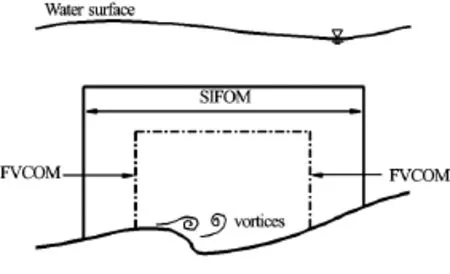
Fig.1 Computational subdomains of the SIFOM-FVCOM system[19]

In FVCOM, a finite volume method is adopted on a triangular mesh in the horizontal plane and a σgrid in the vertical direction. The model has an external mode and an internal mode, their convection terms are approximated using upwind schemes, and the time derivative terms are discretized by Runge-Kutta methods. The external and internal mode may use different time steps. In FVCOM, pressure is not in presence, but it can be recovered by the hydrostatic assumption.FVCOM is now a popular model among coastal ocean community, and its details can be found in Refs.[2,24]. tem are presented in Ref.[19]. The overset grids in the SIFOM-FVCOM system as well as those in SIFOM allow a gradual refinement of mesh resolution from coarse meshes for estuary-scale background tidal flows to fine grids for local flows, providing sufficient flexibility in resolving various phenomena of interests, especially those at small scales.

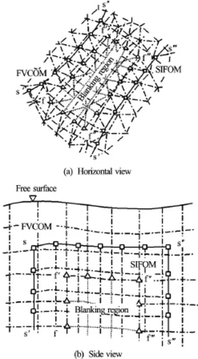
Fig.2 Meshes of the SIFOM-FVCOM system. Squares stand for nodes on an interface of SIFOM, and triangles denote those on an interface of FVCOM

2. Methods for computation of buoyancy

In the SIFOM-FVCOM system, pressure,p , is decomposed into the hydrostatic pressure,ph, and the dynamic pressure,pd. As a result, the governing equations of SIFOM, namely the full, 3D continuity and momentum equations under the Boussinesq approximation, read as[19]

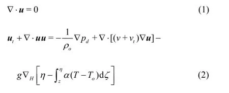
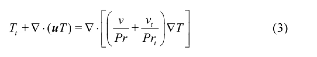
and the equation for heat transfer becomes

In the SIFOM-FVCOM system, SIFOM is coupled with the internal mode of FVCOM, and overset grids are used to integrate the two models, as shown in Fig.2. In this figure, line s-s′-s′′-s′′′andf-f′-f′′-f′′′are model interfaces of SIFOM and FVCOM, respectively. The two models exchange their solutions, such as velocity and pressure, on the interfaces. A linear interpolation is used to obtain boundary conditions for SIFOM at nodes on its interface, e.g., squares in Fig.2, from FVCOM, and a tri-linear interpolation is employed to specify boundary conditions for FVCOM at nodes on its interface, e.g., triangles in the figure. Besides the nodes on the interfaces of the two models, in view of specific features of numerical methods in FVCOM, interpolation is necessary at grid nodes of FVCOM in its blanking zones as shown in Fig.2. The grid of FVCOM deforms with time because water surface elevation keeps changing, and thus a special consideration is necessary for the interpolation procedure. The coupling of SIFOM and FVCOM is in two-way, and a parallel version of the Schwarz iteration is implemented for their solution exchange. The details of the techniques of the SIFOM-FVCOM sys-

In the above equations,u is the velocity vector, and T is the temperature.zis the vertical coordinate of a point in the flow, andηis the water surface elevation above it.g is the gravity,ρoa reference density,Toa reference temperature,athe thermal expansion coefficient,vand vtthe viscosity and the turbulence viscosity, respectively, and Prand Prtthe molecular and the turbulent Prandtl number, respectively. For details, the reader is referred to [19]. Hereafter, Eqs.(1), (2), and (3) are referred to as Type I of SIFOM.

Momentum Eq.(2) is an integro-differential equation, and the computation of the integral on its right hand side is expensive since, at every spatial pointz , it requires an integral from this point to water surface elevation above it. In order to avoid such problem, pressure is decomposed as

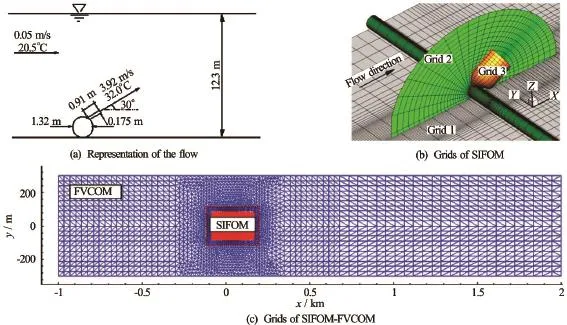
Fig.3 Model setup for the thermal discharge flow

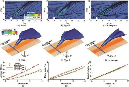
Fig.4 Solutions for the thermal discharge flow

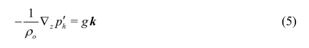
In Eqs.(4) and (5),p′hand pd′are a modification of the hydrostatic and the dynamic pressure, respectively,∇zis the gradient in the vertical direction, andkis the unit vector in the vertical direction. When T=To,andwill reduce to phand pd, respectively. With decomposition (4), momentum Eq.(2) is re-formulated as[19]

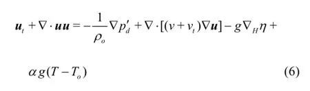
which is a partial differential equation. Eqs.(1), (3) and (6) will be referred to as Type II of SIFOM.

In order to examine the performance of treatment Type I and II of SIFOM, simulation is made for a thermal jet released from a discharge port located on a pipe perpendicular to the longitudinal direction and on the bottom of a straight channel, as shown in Fig.3(a). Details of such flow can be found in Ref.[8]. In computation by SIFOM only, three overset grids with total number of grid nodes 351 770 are used (Fig.3(b)). The computational domain is 75 m in length, 30 m in width, and 12.3 m in height. In computation by SIFOM-FVCOM, FVCOM covers the entire channel, which is 3 000 m in length and 600 m in width, with a mesh that has 7 092 elements in the horizontal plane and 21σ-layers in the vertical direction. SIFOM has four overset grids with 427 929 grid nodes. The flow rate of 369 m3/s is imposed at the inlet of the channel, which corresponds to an inflow velocity of 0.05 m/s, and water surface elevation is fixed as 12.3 m at the outlet.

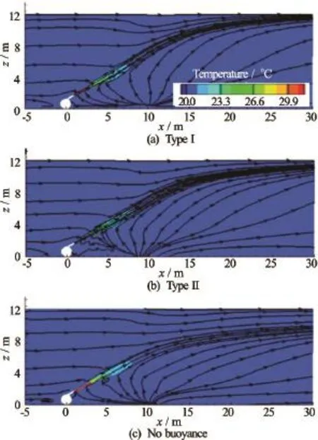
Fig.5 Solutions of the thermal discharge flow obtained with SIFOM-FVCOM

The results computed by SIFOM alone are presented in Fig.4. A solution without buoyancy, which is obtained by turning off the buoyancy terms in Type I and II of SIFOM, is also presented in the figure. Additionally, estimates by CORMIX[25]and Visual Plumes[26]are included. Apparently, the SIFOM’s predictions are closer to the estimate of CORMIX than that of Visual Plumes. A contrast of Fig.4(c) to Figs.4(a) and 4(b) shows the effects of the buoyancy. For instance, the computed streamlines without buoyancy touch the water surface at about x=25 m, while those with buoyancy intersect with the water surface at aboutx=15 m. Overall, the results of SIFOM are in a reasonable agreement with those of CORMIX and Visual Plumes. From these results in the figure, it is seen that Type I and II present correct solutions with similar accuracy.

The solutions obtained with SIFOM-FVCOM are presented in Fig.5, which shows the computed streamlines and temperature at the vertical, centerline cross section. Comparing those in Fig.4, it is seen that SIFOM and SIFOM-FVCOM produce similar but a little different results. The difference is attributed to the fact that the top boundary of the former is a rigid surface while that of the latter is a free surface, in addition to the distinct parameterization of SIFOM and FVCOM. However, it is clearly seen that still solutions produced by Type I and II are close.

Table 1 compares the computational time associated with Type I and II. It is seen that, in case of the SIFOM run, Type I consumes three times of computational time needed by Type II. The time saving by the Type II could be significant in simulations of actual problems when numbers of grid nodes are large. In case of the SIFOM-FVCOM run, the table shows that still Type II consumes less time. However, the saving in time of the SIFOM-FVCOM run is relatively little, only 23%. This is due to the fact that in the SIFOMFVCOM simulation, besides SIFOM, FVCOM and the coupling also consume computational time.

Table 1 Comparison of computation time of Type I and II

In summary, the results in this section indicate that the SIFOM-FVCOM system associated with both Type I and II works. However, Type II presents a solution almost same to that with Type I but is more efficient with regard to computational time. Therefore, Type II is used in the current version of the SIFOMFVCOM system.

3. Lagrangian particle tracking

Lagrangian particle tracking module has been implemented into the present version of the SIFOMFVCOM system. When particles are released fromsites in SIFOM, their paths are computed by SIFOM. As they exit subdomains of SIFOM, their paths will be tracked by FVCOM, even when they return into the SIFOM’s subdomains.

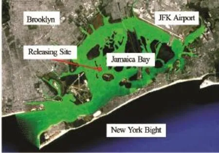
Fig.6 Computational domain and setup for particle tracking in the Jamaica Bay

Fig.7 Particle tracking of estuary flows in Jamaica Bay. Solid lines-trajectories obtained with FVCOM, dashed linestrajectories computed by SIFOM, whose domain is marked as the cubic box in (a)

The SIFOM-FVCOM system is applied to predict the transportation of particles in the Jamaica Bay, as depicted in Fig.6. The computational domain of FVCOM covers the entire Jamaica Bay using 59 881 elements in the horizontal plane and 21σ-layers in vertical direction. The mesh of SIFOM has 35 301 grid nodes, and it covers only a small zone enclosing the releasing site. For purpose of comparison, a computation was also carried out using FVCOM alone.

Figure 7 presents the computed paths of particles near the releasing site, and it shows that the paths computed by SIFOM-FVCOM and FVCOM alone in the SIFOM’s region as well as outside it have certain discrepancy (Figs.7(a) and 7(b)). Nevertheless, after 2 days, the two approaches produce trajectories with substantial difference at the far fields (Figs.7(c) and 7(d)). Therefore, trajectories of fluid particles in a long time are sensitive to local flows where they are released, implying the limitation of using FVCOM alone and necessity to apply the SIFOM-FVCOM system.

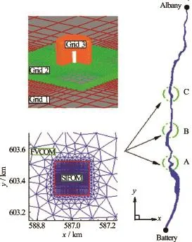
Fig.8 Location of the three piers and computational meshes

4. Simulation of storm surge and its impact on bridge piers

The SIFOM-FVCOM system is applied to model storm surge generated by the Hurricane Sandy in the Hudson River and its impact on three hypothetical bridge piers. The piers are simplified as three cylinders and located at different locations of the river, as shown in Fig.8. In the figure,x,y are the coordinates in UTM, NAD83, and meters, Zone is 18.0, and zis based on the vertical datum NAVD88. The piers are 6 m in height and 2 m in diameter. Each of the cylinders is covered by a SIFOM zone, and FVCOM is applied to the region from the mouth of the HudsonRiver to Albany. FVCOM has 27 462 horizontal elements and 21σ-layers, and the total number of grid nodes for SIFOM at the three cylinders is 917 637, with grid spacing as fine asO(0.01)maround the surface of the piers.

In the simulation, bathymetry data for the Hudson River is from NOAA NGDC, and it is converted to the common vertical datum NAVD88 using NOAA’s VDATUM[27,28]. The river boundaries are specified according to NOAA high-resolution composite vector shorelines[29]. Water surface elevations observed at the Battery station of NOAA NDBC and the Albany station of USGS during Oct. 29th, 2012 to Nov. 1st, 2012, as shown in Fig.9, are respectively used as the upstream and downstream boundary conditions to drive the simulation. The figure indicates that the evolution of elevation in time at the Albany station is about 4 h later than that at the Battery station during the Hurricane Sandy.

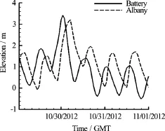
Fig.9 Temporal evolution of water surface elevation observed at the stations of Battery and Albany[30,31]

The simulated all-time highest elevation of water surface along the centerline of the river, together with that of the highest water marks measured at its two banks, is plotted in Fig.10(a). In this figure, the distance starts from the Battery station located at the downstream boundary of the FVCOM’s computational domain. Since the FVCOM’s mesh is relatively coarse in the lateral direction, it cannot appropriately resolve the difference of water surface elevation at the two banks. It is seen that overall the simulation agrees with the measurement with regard to the trends of water surface. They compare well in the range of distance from zero up to 120.7 km, but deviate more within a section after that location. The temporal evolution of the hydrodynamic force on the piers is plotted in Fig.10(b). The small-scale oscillations as shown in the zoom window in this figure are expected to be related to vortex shielding from the piers.

Figure 11(a) shows instantaneous streamlines and velocity distribution computed by FVCOM on the horizontal planes at a moment that the surge propagates in the upstream direction. The simulation by FVCOM provides a view for the large-scale surge flow within the river. Small-scale flow structures around the piers resolved by SIFOM at the corresponding moment are depicted in Fig.11(b). It is seen that there is vortex shielding characterized by many structures small in sizes, and the flow is highly unsteady. It should be noted that the small-scale behaviors of the flow around the piers, e.g., the hydrodynamic force on piers and its small-scale oscillations, can only be captured appropriately by a fully 3-D, fluid dynamics model such as SIFOM, and they are not within the reach of existing coastal ocean models such as FVCOM.

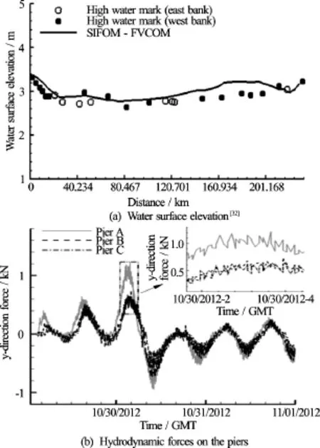
Fig.10 Simulation of storm surge during the Hurricane Sandy

5. Concluding remarks

This paper examines the SIFOM-FVCOM system recently developed for simulation of multiscale and multiphysics coastal ocean flows. In particular, two methods to treat the buoyancy terms in the momentum equations are discussed, and one of them, i.e., Eq.(6), is recommended with regard to its solution accuracy and computational efficiency. Then, an example of particle tracking in Jamaica Bay is presented, and it shows that small-scale flows have effects on large scales of particle trajectories. Finally, the system is applied to compute storm surge within the Hudson River during the Hurricane Sandy, and the simulation simultaneously captures large-scale surge currents as well as small-scale flow behaviors near bridge piers, which is not within the reach of any other existingmodels. All of these results indicate that the SIFOMFOVCOM system works appropriately, and it is a unique, powerful tool for prediction of multiscale and multiphysics coastal ocean flows.

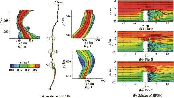
Fig.11 Flow fields on the horizontal plane at z= -15 mwhen the surge propagates upstream, at 3 am, October 30

It is noted that further work should be carried out on strict tests and validations of the SIFOM-FVCOM system, such as quantification of solution accuracy and more detailed analysis of the computational results presented in this paper. In order to assure seamless transition of solutions between SIFOM and FVCOM, it is necessary to design better algorithms at model interfaces, and this may be realized using existing techniques[33-36]. In addition, because that SIFOM has to treat water surfaces as rigid surfaces, and thus it is necessary to develop its capability to deal with free surfaces such as those during waves impact coastal structures. Given its promising performance in example computations, we shall keep these as future topics for study of the SIFOM-FVCOM system.

Acknowledgements

This work was supported by NSF (Grant Nos. CMMI-1334551, DMS-1622459) and PSC-CUNY. Partial support also comes from NSFC (Grant Nos. 51239001, 51509023) and SFMT (Grant No. 2015319825080). The authors are grateful to Dr. C.S. Chen for his input on FVCOM.

[1] Blumberg A. F., Mellor G. L. A description of a threedimensional coastal ocean circulation model (Heaps, N. Three-dimensional coastal ocean models) [M]. Washington, DC, USA: American Geophysical Union, 1987, 1-16.

[2] Chen C., Liu H., Beardsley R. C. An unstructured, finitevolume, three-dimensional, primitive equation ocean model: Application to coastal ocean and estuaries [J]. Journal of Atmospheric and Oceanic Technology, 2003, 20(1): 159-186.

[3] Halliwell G. R. Evaluation of vertical coordinate and vertical mixing algorithms in the hybird coordinate ocean model (HYCOM) [J]. Ocean Modeling, 2004, 7(3-4): 285-322.

[4] Haidvogel D. B., ArangoH., Budgell W. P. et al. Ocean forecasting in terrain-following coordinates: Formulation and skill assessment of the regional ocean modeling system [J]. Journal of Computational Physics, 2008, 227(7): 3595-3624.

[5] Wheeler M. F., Dawson C., Chippada S. et al. Progress report: Parallelization of ADCIRC3D. Technical report [R]. CEWES MSRC Technical Report 98-11. Vicksburg, MS, USA: Waterways Experiment Station, 1988.

[6] Berger M. J., George D. L., LeVeque R. J. et al. The geoclaw software for depth-averaged fows with adaptive refinement [J]. Advances in Water Resources, 2011, 34(9): 1195-1206.

[7] Booij N., Ris R. C., Holthuijsen L. H. A third-generation wave model for coastal regions. 1. Model description and validation [J]. Journal of Geophysical Research, 1999, 104(C4): 7649-7666.

[8] Tang H. S., Paik J., Sotiropoulos F. et al. Three-dimensional numerical modeling of initial mixing of thermal discharges at real-life configurations [J]. Journal of Hydraulic Engineering, ASCE, 2008, 134(9): 1210-1224.

[9] Younis B. A., Teigen P., Przulj V. P. Estimating the hydrodynamic forces on a minitlp with computational fluid dynamics and design-code techniques [J]. Ocean Engineering, 2001, 28(6): 585-602.

[10] Ford R., Pain C. C., Piggott M. D. et al. A nonhydrostatic finite-element model for three-dimensional stratified oceanic flows. Part I: Model formulation [J]. Monthly Weather Review, 2004, 132(12): 2816-2831.

[11] Warner J. C., Geyer W. R., Arango H. G. Using a composite grid approach in a complex coastal domain to estimate estuarine residence time [J]. Computers and Geosciences, 2010, 36(7): 921-935.

[12] Debreu L., Marchesiello P., Penven P. et al. Two-way nesting in split-explicit ocean models: Algorithms, implementation and validation [J]. Ocean Modelling, 2012, 49-50(3): 1-21.

[13] Fringer O. R., McWilliams J. C., Street R. L. A new hybrid model for coastal simulation [J]. Oceanography, 2006, 19(1): 64-77.

[14] Choboter P. F., Garcia M., Cecchis D. D. et al. Nesting nonhydrostatic GCCOM within hydrostatic ROMS for multiscale coastal ocean modeling [C]. Oceans16 MTS IEEE. Monterey, CA, USA, 2016.

[15] Fujima K., Masamura K., Goto C. Development of the 2D/3D hybrid model for tsunami numerical simulation [J]. Coastal Engineering Journal, 2002, 44(4): 373-397.

[16] Sitanggang P. J., Lynett K. I. Multi-scale simulation with a hybrid boussinesq-rans hydrodynamic model [J]. International Journal for Numerical Methods in Fluids, 2009, 62(9): 1013-1046.

[17] Tang H. S., Wu X. G. Multi-scale coastal flow simulation using coupled CFD and GFD models. Modelling for environment’s sake [C]. Fifth Biennial Meeting. Ottawa, Canada, 2010.

[18] Wu X. G., Tang H. S. Coupling of CFD model and FVCOM to predict small-scale coastal flows [J]. Journal of Hydrodynamics, 2010, 22(5 Suppl.): 284-289.

[19] Tang H. S., Qu K., Wu X. G. An overset grid method for integration of fully 3D fluid dynamics and geophysics fluid dynamics models to simulate multiphysics coastal ocean flows [J]. Journal of Computational Physics, 2014, 273: 548-571.

[20] Tang H. S., Qu K., Wu X. G. et al. Domain decomposition for a hybrid fully 3D fluid dynamics and geophysical fluid dynamics modeling system: A numerical experiment on a transient sill flow [C]. Domain Decomposition Methods in Science and Engineering XXII, Lecture Notes in Computational Science and Engineering. Lugano, Switzerland, 2016, 407-414.

[21] Lin F. B., Sotiropoulos F. Assessment of artificial dissipation models for three-dimensional incompressible flows [J]. Journal of Fluids Engineering, 1997, 119(2): 331-340.

[22] Tang H. S., Jones C., Sotiropoulos F. An overset-grid method for 3D unsteady incompressible flows [J]. Journal of Computational Physics, 2003, 191(2): 567-600.

[23] Ge L., Sotiropoulos F. 3D unsteady RANS modeling of complex hydraulic engineering flows. I: Numerical model [J]. Journal of Hydraulic Engineering, ASCE, 2005, 131(9): 800-808.

[24] Lai Z., Chen C., Cowles G. et al. A non-hydrostatic version of FVCOM, Part I: Validation experiments [J]. Journal of Geophysical Research, 2010, 115: C11010.

[25] Jirka G. H., Doneker R. L., Hinton S. W. User’s manual for CORMIX: A hydrodynamic mixing zone model and decision support system for pollutant discharges into surface waters [R]. New York, USA: DeFrees Hydraulics Laboratory, Cornell University, 1996.

[26] Frick W. E., Roberts P. J. W., Davis L. R. et al. Dilution models for effluent discharges [M]. 4th Edition, Washington, DC, USA: U.S. Environmental Protection Agency, 2003.

[27] NOAA NGDC. Bathymetric data viewer [EB/OL]. http://maps.ngdc.noaa.gov/viewers/bathymetry/.

[28] NOAA. Vertical datum transformation [EB/OL]. http://vdatum.noaa.gov/.

[29] NOAA Coastal Services Center. NOAA composite coastline [EB/OL]. http://shoreline.noaa.gov/data/datasheets/composite.html.

[30]NOAA NDBC [EB/OL]. http://www.ndbc.noaa.gov/.

[31]USGS. WaterAlert [EB/OL]. http://water.usgs.gov/wateralert/.

[32] USGS. Hurricane Sandy storm-surge high-water-marks [EB/OL]. http://ny.water.usgs.gov/flood/HudsonSandy. JPG.

[33] Berger M. J. On conservation at grid interfaces [J]. SIAM Journal on Numerical Analysis, 1987, 24(5): 967-984.

[34] Tang H. S., Zhou T. On non-conservative algorithms for grid interfaces [J]. SIAM Journal on Numerical Analysis, 1999, 37(1): 173-193.

[35] Tang H. S. Study on a grid interface algorithm for solutions of incompressible Navier-Stokes equations [J]. Computers and Fluids, 2006, 35(10): 1372-1383.

[36] Foster N. F. Accuracy of high-order CFD and overset interpolation in finite volume/difference codes [C]. 22nd AIAA Computational Fluid Dynamics Conference. Dallas, TX, USA, 2015, AIAA Aviation, AIAA 2015-3424.

(Received June 24, 2016, Revised September 3, 2016)

* Biography:K. QU, Male, Ph. D. Candidate, Research Assistant

Hansong TANG,

E-mail: htang@ccny.cuny.edu