Collaborative Simulation Method with Spatiotemporal Synchronization Process Control
2016-12-09ZOUYishengDINGGuofuZHANGWeihuaZHANGJianQINShengfengandTANJohnKian
ZOU Yisheng, DING Guofu, , ZHANG Weihua, ZHANG Jian, QIN Shengfeng, 3, and TAN John Kian
Collaborative Simulation Method with Spatiotemporal Synchronization Process Control
ZOU Yisheng1, DING Guofu1,*, ZHANG Weihua2, ZHANG Jian1, QIN Shengfeng1, 3, and TAN John Kian4
1 School of Mechanical Engineering, Southwest Jiaotong University, Chengdu 610031, China;2 State Key Laboratory of Traction Power, Southwest Jiaotong University, Chengdu 610031, China;3 Northumbria School of Design, Northumbria University, Newcastle upon Tyne NE1 8ST, UK;4 School of Mechanical and Construction Engineering, Northumbria University, Newcastle upon Tyne NE1 8ST, UK
When designing a complex mechatronics system, such as high speed trains, it is relatively difficult to effectively simulate the entire system’s dynamic behaviors because it involves multi-disciplinary subsystems. Currently,a most practical approach for multi-disciplinary simulation is interface based coupling simulation method, but it faces a twofold challenge: spatial and time unsynchronizations among multi-directional coupling simulation of subsystems. A new collaborative simulation method with spatiotemporal synchronization process control is proposed for coupling simulating a given complex mechatronics system across multiple subsystems on different platforms. The method consists of 1) a coupler-based coupling mechanisms to define the interfacing and interaction mechanisms among subsystems, and 2) a simulation process control algorithm to realize the coupling simulation in a spatiotemporal synchronized manner. The test results from a case study show that the proposed method 1) can certainly be used to simulate the sub-systems interactions under different simulation conditions in an engineering system, and 2) effectively supports multi-directional coupling simulation among multi-disciplinary subsystems. This method has been successfully applied in China high speed train design and development processes, demonstrating that it can be applied in a wide range of engineering systems design and simulation with improved efficiency and effectiveness.
design automation, collaborative simulation, space and time synchronization, process control, coupling algorithms, mechatronic system design
1 Introduction
Efficient engineering product design and analysis methods and tools play an important role in supporting rapid product development to meet mass-customization requirements in Industry 4.0 era. Particularly when designing a complex mechatronics system with multiple subsystems, the whole system dynamic simulation plays a key role in product system design and development. The challenges in conducting system dynamic simulation include 1) how to model the entire system’s dynamics behaviors and interactions by incorporating all the subsystems’ behaviors possibly from multi-disciplinary fields, and 2) how to effectively simulate such a complex multi-disciplinary system’s behaviors.
At present, multi-disciplinary simulation has attracted attentions from scholars and researchers. Kübler and Schiehlen[1–2]proposed a modular formulation of multibody systems(MBS) based on the block representation of a multibody system with corresponding input and output quantities to facilitate exchanges and integrations of results among different software for each module/subsystem. It provides two simulator coupling methods, namely the iteration method and filter method, to resolve the problems in which the coupling of simulators may result in an unstable integration. Krüger, et al[3–4], based on SIMPACK(a MBS-based system), proposed a multidisciplinary simulation method to combine different CAE tools, like FEA, CAD, and CACE, allowing the computation and evaluation of a complex system with the desired accuracy and within acceptable computation times.Liang, et al[5]proposed a combinative algorithm for communication among domain models in multidisciplinary collaborative simulation by using a proper model encapsulation method and a matched RTI control strategy. Arnold, et al[6–9], discussed multidisciplinary simulation problems and the relevant algorithms used in both mono and multi-disciplinary simulation of vehicle system dynamics, presented some numerical methods together with estimation of errors for coupling simulation, and developed the Functional Mock-Up Interface(FMI) for supporting multi-disciplinary modeling and simulation. Huang, et al[10], studied the algebraic loop problem in multi-domain simulation to reveal the relationship between simulation stability and system topologies, and proposed two algebraic loop compensation algorithms using both numerical iteration and approximate function to simulate the forging process. LI, et al[11], applied a collaborative simulation based on interfaces to a tracked vehicle.
In the field of multi-disciplinary simulation for complex mechatronics systems, there are two typical methods: close coupling simulation and weak coupling simulation[4]. Close coupling means all subsystem models are built up and solved by a unified method, while weak coupling means all subsystems are modeled and solved independently, and they are coupled by interfaces. Nowadays, close coupling simulation using Modelica is a trend[12]. Modelica is recognized as a universal language for modeling and simulation in engineering, which could build and combine a complex system through object-oriented manner. It is a promising modeling method[13–14], and spread successively by many commercial software(such as CATIA,SIMPACK and LMS VIRTUAL LAB). For example, Dymola developed by CATIA promotes the study on the modeling and simulation of complex mechatronics systems, along with others such as LMS AMESim, SIMPACK/Dymola, JModelica.org, MapleSim, MathModelica, OpenModelica and so on[15]. Modelica has a flexible modeling approach, but model library needs to be further developed. So far, it is difficult to build a complex and dynamics coupled system like high speed train by this way, because of its characteristics in system composition, modeling method, integration method and coupling manners. In addition, solving the coupled system dynamics based on commercial software and Modelica, requires a unified integration method and it is hard to find a unified integration method to solve all forms of dynamics systems, which include hydrodynamics, rigid body dynamics, flexible body dynamics, etc.
Interface based weak coupling simulation is the most practical approach for multi-disciplinary simulation, which uses commercially available software to analyze system inputs, outputs, boundary conditions, etc., and then defines a co-simulation mode, such as the combined simulation of ABAQUS, SIMPACK, ADAMS, MATLAB/SIMULINK, FLUENT, and LMS[16–18], or under the collaborative simulation architecture of HLA/RTI[19]. Most recent researches on this method mainly focus on the uni-directional or bi-directional[4]coupling simulation between two subsystems in a single platform(shown in Fig. 1) such as PC1 with Windows system, while many mechatronics systems(eg. train) generally include more than two subsystems with multi-directional interactions (either uni-directional(Uni-) or bi-directional(Bi-) in Fig 1(c)), and these subsystems usually operates on different platforms such as PC1 and PC2 with Windows system and high performance computer-HPC1 with Linux system as shown in Fig. 1(c). The use of multiple different platforms in a distributed computing environment can improve the computing efficiency by parallel computing but meanwhile it causes more process control problems during coupling simulation, such as how to prepare and generate boundary data for data exchanges among related subsystems, how to implement fast and reliable data exchange and how to control the simulation process to meet the spatiotemporal synchronization requirement across multiple subsystems on different platforms.
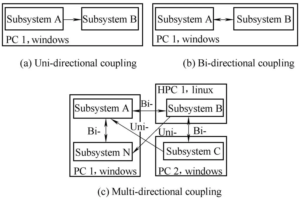
Fig. 1. Problem definition of coupling simulation
Here an interface based multi-disciplinary collaborative simulation method with spatiotemporal synchronization process control that can solve mentioned problems and support complex dynamics design, simulation and design automation is proposed. Firstly, a component-and-coupler based modeling method is developed to define and package the entire system easily and flexibly with clear relationship definitions among subsystems. This system model and definition can guide the boundary data preparation for related subsystems and suggest data exchange mechanisms based on involved subsystems’ platforms and simulation coupling requirements. Secondly, a new spatiotemporal synchronization process control algorithm is proposed to efficiently coordinate sub-systems with different simulation steps(resulting in asynchronous space) and different simulation times per step(leading to asynchronous time) in a cross-platform, cross-system and multi-disciplinary computing environment. Thirdly, a linear forward and backward interpolation method is adopted to obtain the desired accuracy of boundary data of related subsystems in affordable computation times. Finally, data check and data transfer confirmation mechanism based the user datagram protocol(UDP) is implemented to improve efficiency and reliability of data transmission in cross platform coupling simulation.
The remainder of the paper is structured as follows. Section 2 introduces the component-based subsystem simulation modeling. The new collaborative simulation method with spatiotemporal synchronization process control is described in section 3, followed by a case study in section 4. Final conclusions are drawn in section 5.
2 Component-and-coupler Based Collaborative Simulation Method
The proposed new simulation method consists of a component-and-coupler based coupling mechanism(see Fig. 2) and a simulation process control algorithm based on spatiotemporal synchronous integral. In computing terms, a component means a simple encapsulation of datum and methods. Methods are some simple and visible functions of the component. Object-oriented design can be really realized with the component concept. With this method, a component can be treated as a black box(without loss of generality and functionality), the users just need to comprehend its mechanism, so that its internal working process can be ignored. The component-based modeling method therefore offers flexibility to allow coupling calculation models with various coupling levels to be established quickly.

Fig. 2. Component-and-coupler based coupling mechanism for distributed collaborative simulation
A very complex mechatronics system can now be modelled with many components(subsystems) and each component can be described by a simulation model with its input/output interfaces. The interactions among these components can be described and facilitated by the coupler (or coordinator). Note that there are differences among different subsystems’ simulation models. Firstly, the simulation calculations are performed in different simulation supporting environments. Secondly, the modeling method, integration method, simulation step size and one-step simulation time are all different in various simulation calculation models. Therefore, the key issue to be addressed is the coordination of these simulation components in a unified computing platform to achieve spatial and temporal synchronization. The solution is presented in Fig. 2 and details are as follows:
(1) Step 1(S1), the user creates a simulation project, then prepare simulation input files of each sub-system, and submit a coupling simulation task to the scheduler.
(2) Step 2(S2), the scheduler receives the task and then downloads the input files of each sub-system to the computer which models the component. At the same time, the scheduler will write and download a configuration file to each sub-system. The file records the simulation information such as project number, ip address and port of coupler, input and output interfaces, simulation step size, ip address and port of sub-system, etc.
(3) Step 3(S3), the scheduler downloads the coupling simulation information of this task and sends a message to the coupler to start the simulation. The coupling simulation information is also written in a configuration file, which includes the project number, coupling modules, coupling relationship and interfaces among all modules, ip address and port of the coupler, simulation time, etc.
(4) Step 4(S4), the coupler receives and decodes the configuration file, sends message to all components to start the coupling simulation. A spatiotemporal synchronous integral algorithm is used to control the coupling simulation process and exchange the interfaces data.
(5) Step 5(S5), when the coupling simulation is completed, the coupler will send result information to the scheduler, and then scheduler will finish the simulation task and recycle its computing resources.
(6) Step 6(S6), the scheduler sends task result messages to the user interface and the user can review the simulation results.
The coupler is the key to link each sub-system and carry out the coupling calculations. It coordinates and synchronizes simulation processes of each sub-system spatiotemporally. By solving the coupling relationship model of the coupled system dynamics, it updates the simulation boundary conditions of each sub-system and drives the relevant sub-systems to couple or work with each other, so that the coupling multiple sub-systems can generate their simulation results in an efficient and effective way. The main functions of the coupler are as follows:
(1) Controlling the coupling simulation process, such as the startup, wait and stop of each coupled sub-system;
(2) Building simulation models correspondingly to carry out a fully or partially coupling simulation according to the user demand;
(3) Coordinating simulation processes of sub-systems to realize coupling calculations by some designed strategies (such as multi-level simulation step synchronized coordination strategy and virtual timeline based simulation time synchronized coordination strategy) because of the different sizes of simulation step and time among sub- systems;
(4) Processing coupling simulation boundary conditions data of subsystems at coupling step by using some designed algorithms(such as data interpolation algorithm) for mitigating the change of boundary conditions to ensure the stability and accuracy of the coupling simulation, which provides input data for current step calculation of each sub-system;
(5) Collecting and distributing simulation boundary conditions data of subsystems by communicating with the coupling sub-systems in real time, including receiving the output date from coupling sub-systems, and sending the processed simulation boundary conditions data to the coupling sub-systems to update its input.
This coupling mechanism can also support distributed and parallel computing for computer based collaborative work, which can improve the efficacy of the simulation with reduced computational time. Multiple couplers could be deployed to ensure the load balancing of the whole simulation system.
3 Spatiotemporal Synchronization Process Control Algorithm
The coupling simulation system consists of multiple subsystems, the component-based modeling strategy is used to coordinate subsystems’ simulations within the entire system simulation and in the meanwhile reduce the complexity of system wide modeling and simulation. However, in this collaborative simulation method, each subsystem is relatively domain independent, and their behavior functions are different, so different integral step of each subsystem is required to make their states and behavior simulations smooth and steady. The goal of each subsystem simulation is to obtain its state and behavior information by time integral. Each subsystem performs its simulation at its own integral step size within the time domain. Therefore, at the end of an integral step, their positions are inconsistent due to their different integral step sizes. This is the problem of spatial unsynchronization. It is true if a consistent minimal integral step crossing all subsystem is used, all subsystems can be coordinated in this way to avoid this spatial unsynchronization problem, but this will cause a computational efficiency problem because some subsystems will do integral computing several times instead of doing it once to achieve a required result. Therefore, the spatial synchronization of each subsystem is a core problem to be solved in this paper.
In addition to the spatial unsynchronization problem, another core problem is time unsynchronization problem. When a subsystem performs an one-step integral, the computational time is different and to arrive at a given position, the subsystem also requires a different number of integration steps. Let a subsystem Si spendscomputational time to complete one-step integration and for approaching to a common spatial position to exchange information among all subsystems and conduct a next round collaborative simulation, the subsystem requiresintegration steps. Therefore, the subsystem Si needs a total computational time:. Obviously, each subsystem needs different computational times to reach the common position. This leads to the time unsynchronization problem.
In principle, integrating multiple subsystems into a collaborative simulation requires all subsystems to work together in a spatiotemporal synchronous manner because a subsystem needs inputs from other related subsystems with a common spatiotemporal reference point such as a position in a physical environment. In reality, the integral step of each sub-system can be different. The core of component-based coupling simulation of multiple subsystems is exchanging state and behavior data among relative subsystems at given positions and driving them to start the next or following step simulation together, so the spatiotemporal synchronization process control is necessary to achieve this.
Some simulation systems may use variable integral steps to improve efficiency and precision. In this case, it is difficult to setup some fixed steps to control a coupling simulation process because each integral step of a subsystem is dynamic. Here a possible solution to this problem is presented.
Three hypothetical subsystems A, B, and C are taken as an example for controlling coupling simulation. As shown in Fig. 3, the system includes subsystems A, B and C, the permissible minimal integral steps of each subsystem are defined as Min_stepA, Min_stepB and Min_stepC, the integral steps are defined as StepA(from 1 to), StepB(from 1 to), StepC(from 1 to), the accumulated steps are defined as AccstepA, AccstepB and AccstepC. The minimal control step of coupled simulation system is defined as Ctrlstep, the accumulated step is defined as AccSimustep, the simulation time is defined as Simutime.

Fig. 3. Coupled control method for subsystems with variable integral steps
The control algorithm is as follows.
(1) Ctrlstep=min(Min_stepA,Min_stepB,Min_stepC);
AccstepA += StepA 1;
AccstepB += StepB 1;
AccstepC += StepC 1;
Subsystem A,B,C setup and simulate one step;
Subsystem A,B,C send interface data to coupler;
(2) for(i=1; AccSimustep<=Simutime; i++)
{ AccSimustep = i*Ctrlstep;
if(AccSimustep>= AccstepA)
{ receive interface data from coupler;
Subsystem A simulates one step;
Send interface data to coupler for next step simulation;
AccstepA += StepA i;
}
if(AccSimustep>= AccstepB)
{ receive interface data from coupler;
Subsystem B simulates one step;
Send interface data to coupler for next step simulation;
AccstepB += StepB i;
}
if(AccSimustep>= AccstepC)
{ receive interface data from coupler;
Subsystem C simulates one step;
Send interface data to coupler for next step simulation;
AccstepC += StepC i;
}
}
From Fig. 3, it is not difficult to see that the coupling interface data need further treatment because the integral steps of each subsystem are dynamic and they are not integral multiple. In Fig. 3, subsystem A needs the coupling interface data from subsystem B to finish one-step simulation. Here subsystem A and B are taken as example to explain the processing algorithm:
(1) The first step, the coupling interface data is initialized by the coupler, subsystems A and B receive the coupling interface data from the coupler and finish this step simulation, and then send new interface data to the coupler for next step simulation.
(2) When subsystem A begins the second step simulation, the coupling interface data from subsystem B should be prepared and ready for use. But on the integral space axis, it can be found that the space of interface data of subsystem B is at the right of the beginning space point of subsystem A. It is a spatial unsynchronization problem, caused by different integral steps. In order to get the interface data for subsystem A’s second step simulation, the coupler should use a linear forward interpolation method between the initialized interface data and the first step interface data of subsystem B.
(3) When subsystem A begins the third step simulation, it can be found that the space of interface data of subsystem B is at the left of the beginning space point of subsystem A. In this case, the coupler should use a linear backward interpolation method between the first interface data and the second step interface data of subsystem B to obtain the necessary data.
The variable integral steps may speed up the simulation process, but some estimated interface data such as from backward or forward interpolation may affect the quality of the simulation.
In a distributed collaborative simulation, subsystems’ calculating process and simulation synchronous controlling are based on network communications. The data transmission and simulation synchronous controlling among sub-systems are realized by the fast and steady communication function between the sub-system executors (used for simulation calculation of the sub-systems) and the coupler, which is on the base of the user-defined private protocol encapsulated by UDP(User Datagram Protocol). As UDP with low reliability, a data check and retransmission mechanism is designed in coupler and executors. In a given time point, the coupler(or executor) checks whether the coupling data from executor (or coupler) is arrived successfully. If not, the coupler(or executor) will require the executor(or coupler) to retransfer the coupling data. This method keeps the reliability and improves the efficiency of distributed collaborative simulation.
Simply put, the coupler is the transfer station of data. For ensuring reliability and transparency in data access, the sub-system executors send the coupling data(used by other subsystems) of current step to the coupler, and then queries the necessary coupling input data (from other subsystems) for next step simulation from the coupler. If the coupling input data are by then prepared and ready for use, the executor of this sub-system gets the coupling input data from the coupler for next step simulation calculation; otherwise, the sub-system keeps on waiting and querying until the coupling input data is ready.
4 Simulation Case Study and Analysis
4.1 Component-based simulation model for a high speed train
To verify the validity of the proposed simulation method, a coupling simulation case has been studied with sub-systems of the vehicle dynamics, track dynamics and aerodynamics of a high-speed train, as shown in Fig. 4. The subsystem models are described in detail below.
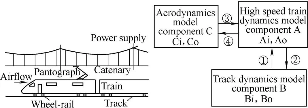
Fig.4. High speed train-track-airflow coupled modeling
In this case study, a vehicle dynamics model of a certain CRH vehicle is first established. The vehicle dynamics system includes one car body, two frames, eight axle boxes and four wheel sets, in total there are 15 bodies with correspondingly 42 degrees of freedom(DOF). The primary suspension includes steel spring, vertical damper etc., and the tumbler positioning mode is adopted. The secondary suspension includes air spring, lateral backstop, lateral damper, anti-hunting damper, traction rod, etc. In the established multi-body model of vehicle dynamics, the car body, frames, axle boxes and wheel sets are defined as rigid bodies. Force element models are established according to the positions and performance characters of the components of the primary and secondary suspension. A developed system is adopted for building the vehicle dynamics sub-model A.
In the wheel-rail relation model, an improved trace method is adopted to seek the wheel-rail contact points quickly, non-linear hertz spring theory is utilized to calculate the wheel-rail normal force, and the Shen’s theory is adopted to calculate the wheel-rail creep force. Combined with the look-up table method and real-time calculation method, the wheel-rail forces can be calculated relatively quickly and precisely. For this simulation, the Jingjin track spectrum[20]is adopted as the typical track irregularity input data.
The vehicle and the track are two indivisible major parts of the railway transportation system. The vehicle system and the track system are not isolated, but mutual coupled with interactions[21].
In this case study, Zhai’s model[21–22]is adopted as the track dynamics model. In the model, the rail is defined as a Bernoulli-Euler beam supported by elastic points, the interval of rail supporting points is the interval of fasteners, the track slab and pedestal of slab ballastless track are defined as thin elastic plates on elastic foundation, and the continuous casted ballastless track is defined as a discrete model. A developed system is adopted for building the track dynamics sub-module B, and the relevant parameters are shown in Table 1.

Table 1. Major parameters of slab ballastless track
A train is a relatively huge and long object, whose head and tail are constituted of many curved surfaces with different curvatures. In addition, its surfaces are not perfectly smooth aerodynamically because of the pantograph and the bottom structure of the vehicle. With increasing running speed, air resistance of the train increases sharply in accordance to the law of aerodynamics. In addition many traffic safety and surrounding aerodynamics problems appeared[23].
In this case study, the commercial software Fluent was adopted for building the vehicle aerodynamics sub-model C. Fig. 5 is the aerodynamics model for the case in section 4.3.1, which compares the simulation result with the experimental result when two trains meeting. In this case, the size of computing area is 500 m´200 m´40 m, and the distance between two trains is 5 m.
Fig. 6 presents the aerodynamics model for the case in section 4.3.2, which compares the simulation results between traditional method and coupling method (proposed by this paper) when a train operating under the condition of cross wind. In this case, the size of computing area is 350 m´90 m´60 m, the distance between the entrance and the front tip of the vehicle head is 100 m, the distance between the export and the front tip of the vehicle head is 175 m, the distance between the entrance of windward side and the track center line is 30 m, the distance between the export of leeward side and the track center line is 60 m, the distance between the vehicle and the ground is 0.376 m.

Fig.5. Aerodynamics model of two trains meeting
Fig.6. Aerodynamics model of high speed train with the action of cross wind
4.2 Coupling simulation controlling parameters
According to the simulation calculation model shown in Fig. 4, the calculation parameters for the sub-systems and the coupling simulation controlling parameters are then set up accordingly. Considering the efficiency and accuracy of simulation of subsystems, the integration step of the vehicle dynamics sub-system A and track dynamics sub-system B are set as 5´10–5s, and 2´10–3s for the aerodynamics sub-system C. Then according to the spatiotemporal synchronization process control algorithm, the coupled simulation controlling step for the first layer will be automatically set as 5´10–5s, and 2´10–3s for the second layer.
4.3 Results validation
When two high speed vehicles travel pass each other (“meeting”) in relative close proximity the air flow between the two vehicles is complex, and a powerful transverse impact force is generated as a result, this transversely induced impact force tends change the posture of the vehicles. The impact can be detected with relative ease by a vibration acceleration sensor mounted on the vehicles. Therefore, for this reason this condition is used as a typical test condition to be analyzed by coupling simulation, the result of which can be validated with experimental data. This is the validation approach adopted by this case study to verify the validity of the proposed collaborative simulation method. The accuracy of the simulation calculation is verified by comparing the simulated results with the measured results of vehicle dynamics index (transverse vibration acceleration of car body) in this meeting condition. The running speed of the meeting trains was 350 km/h, and the simulation and experiment results are shown in Fig. 7.

Fig. 7. Transverse vibration acceleration of left-front test point on carbody of head train with meeting speed of 350km/h
From Fig. 7, it can be clearly seen that the trend of the simulation result and the experiment result is consistent, but the amplitude of simulation result is slightly smaller than experimental result; this difference could be explained by the use of a simplified vehicle and track model during simulation. The meeting time interval is different because there were 3 vehicles in simulation and 8 vehicles in experiment. These differences will not affect the validity of the simulation results and hence it can be stated with confidence that the result demonstrated the validity of the proposed collaborative coupled simulation method.
When the train is running, the resistance, lift force and lateral force generated by its surrounding airflow will affect the posture of the vehicle. In turn, the posture change of the vehicle will affect the distribution of its surrounding airflow field. This is a coupling process which cannot be reflected by traditional aerodynamic and vehicle dynamics simulation. The differences in terms of results between the coupling simulation models and traditional simulation methods are presented by modeling the force of high speed train with the effect of cross-wind. For this comparison, the vehicle run in a straight rail at the speed of 350 km/h under the cross-wind condition, the wind speed was 5 m/s.
Two methods of analysis were performed: Solution 1 adopted the vehicle-track-airflow coupling model and simulation algorithm proposed by the paper, while Solution 2 adopted the traditional aerodynamics simulation method.
The simulation results of the lift force and lateral force of the head vehicle from two solutions are shown in Fig. 8. The traditional aerodynamic can obtain only the steady state force of the vehicle with the effect of cross-wind, while the coupling system dynamics can obtain the transient state force. More importantly the simulation result is consistent with the theoretical analysis result in terms of the overall profile of the performance, which further verifies the validity of coupling simulation models and coupling simulation calculating methods.

Fig.8. Simulation results of traditional aerodynamic andvehicle-track-airflow coupled dynamics
5 Conclusions
(1) The proposed collaborative simulation method has been proven to be able to effectively support multi-directional coupling simulation among complex multi-disciplinary subsystems.
(2) The proposed method composes of generic algorithms, thus technically it can well support distributed, scalable and parallel computing for the coupling simulation of complex vast system.
(3) A further advantage of this method is that it can be implemented in a distributed computing environment.
(4) This method has been successfully applied in simulating coupled vast system dynamics of a high-speed train. The coupling computation among multi sub-systems of high speed train is realized effectively by solving the coupling relationship model with the corresponding spatiotemporal synchronization process control algorithm.
(5) Under Industry 4.0 era and beyond, efficient and effective product dynamic behavior simulation methods are very demanding to make rapid new product development to meet dynamic market changes and better user experiences. Thus, the proposed new complex product design and simulation method has a potential to be applied in a wide application field.
[1] Kübler R, Schiehlen W. Modular simulation in multibody system dynamics[J]., 2000, 4: 107–127.
[2] Kübler R, Schiehlen W. Two methods of simulator coupling [J]., 2000, 6(2): 93–113.
[3] Krüger W R, Vaculin O, Kortüm W. Multi-disciplinary simulation of vehicle system dynamics[C]//, Paris, France, April 22–25, 2002: 1–16.
[4] Vaculin O, Krüger W R, Valášek M. Overview of coupling of multibody and control engineering tools[J]., 2004, 41(5): 415–429.
[5] Liang Silv, Zhang Heming. A novel combinative algorithm for multidisciplinary collaborative simulation[C]//, Xi’an, China, April 16–18, 2008: 104–109.
[6] Arnold M, Carrarini A, Heckmann A, et al. Simulation techniques for multidisciplinary problems in vehicle system dynamics[J]., 2003, 40(Supp.): 17–36.
[7] Schierz T, Arnold M, Clauß C. Co-simulation with communication step size control in an FMI compatible master algorithm[C]//, Munich, Germany, September 3–5, 2012: 205–214.
[8] Arnold M, Clauß C, Schierz T. Error analysis and error estimates for co-simulation in FMI for model exchange and co-Simulation v2.0[J]., 2013, LX(1): 75–94.
[9] Arnold M, Hante S, Köbis M A. Error analysis for co-simulation with force-displacement coupling[J]., 2014, 14(1): 43–44.
[10] HUANG Shunzhou, ZHAO Yong, WANG Hao, et al. Stabilized multi-domain simulation algorithms and their application in simulation platform for forging manipulator[J]., 2014, 27(1): 92–102.
[11] LI Sanqun, HU Zhongling, JIA Changzhi, et al. Research on multi-disciplinary collaborative simulation based on interfaces used in tracked vehicle[C]//, Hangzhou, China, September 28–29, 2015:547–552.
[12] Mattsson S E, Elmqvist H, Broenink J F. Modelica: an international effort to design the next generation modeling language[C]//, Gent, Belgium, April 28–30, 1997: 16–19.
[13] Zhang Jian, Peng Xiaobo. Research on Modelica based modeling and simulation of PCB AOI imaging system[C]//, Shenyang, China, APR 24–26, 2015: 1159–1164.
[14] Otter M. Multi-domain modeling and simulation[C]//, London: Springer, 2015: 805–816.
[15] Erdélyi H, Prescott W, Donders S, et al. FMI implementation in LMS Virtual.Lab Motion and application to a vehicle dynamics case[C]//, Munich, Germany, September 3–5, 2012: 759–764.
[16] NIE YiZhao, ZENG Jing, LI FanSong. Research on resonance vibration simulation method of high-speed railway vehicle carbody[C]//, Xi’an, China, JAN 10–11, 2015: 1117–1121.
[17] Brezina T, Hadas Z, Vetiska J. Using of co-simulation ADAMS-SIMULINK for development of mechatronic systems[C]//, Trencianske Teplice, Slovakia, June 1–3, 2011: 59–64.
[18] Spitans S, Baake E, Nacke B, et al. Numerical modeling of free surface dynamics of melt in an alternate electromagnetic field[J]., 2016, 47(1): 522–536.
[19] YUE Yingchao, FAN Wenhui, XIAO Tianyuan, et al. Novel models and algorithms of load balancing for variable-structured collaborative simulation under HLA/RTI[J]., 2013, 26(4): 629–640.
[20] TPL.[R]. Chengdu: Traction Power State Key Laboratory of Southwest Jiaotong University, 2008. (in Chinese)
[21] Zhai Wanming.[M]. 3rd ed. Beijing: China Railway Publishing House, 2007. (in Chinese)
[22] Cai Chengbiao.[D]. Chengdu: Southwest Jiaotong University, 2004. (in Chinese)
[23] Cui Tao, Zhang Weihua. Study on safety of train in side wind with changing attitudes[J]., 2010, 32(5): 25–29. (in Chinese)
Biographical notes
ZOU Yisheng, born in 1980, is currently an associate research fellow at. He received his PhD degree from, in 2009. His research interests include multi-disciplinary simulation and digital design.
Tel: +86-28-87601538; E-mail: zysapple@sina.com
DING Guofu, born in 1972, is currently a professor at. He received his PhD degree from, in 2000.His research interests include digital design and intelligent manufacturing.
Tel: +86-28-87601643; E-mail: dingguofu@163.com
ZHANG Weihua, born in 1961, is currently a professor at. His research interests include dynamics of coupled system in high-speed train and pantograph/catenary system dynamics.
E-mail: tpl@home.swjtu.edu.cn
ZHANG Jian, born in 1972, is currently an associate professor at. She received her PhD degree from, in 2015.Her research interests include digital design and optimization.
E-mail: 527733@qq.com
QIN Shengfeng, born in 1962, is currently a professor at. He received his PhD degree from, in 2000. His research interests include digital design and product/industrial design.
E-mail: sheng-feng.qin@northumbria.ac.uk
TAN John Kian, is currently a subject leader atHis main research interests include data analysis, safety/risk analysis, multiple criteria decision making and engineering design.
E-mail: k.tan@northumbria.ac.uk
Supported by National High Technology Research and Development Program of China(863 Program, Grant No. 2015AA043701-02)
© Chinese Mechanical Engineering Society and Springer-Verlag Berlin Heidelberg 2016
Received May 12, 2016; revised August 2, 2016; accepted August 5, 2016
10.3901/CJME.2016.0805.088, available online at www.springerlink.com; www.cjmenet.com
E-mail: dingguofu@163.com
杂志排行

Chinese Journal of Mechanical Engineering的其它文章
- Surface Topography and Roughness of High-speed Milled AlMn1Cu
- Exploring Local Regularities for 3D Object Recognition
- Engineering the Smart Factory
- Exploring Barriers and Opportunities in Adopting Crowdsourcing Based New Product Development in Manufacturing SMEs
- Development of the Supply Chain Oriented Quality Assurance System for Aerospace Manufacturing SMEs and Its Implementation Perspectives
- Simulation Based Energy-resource Efficient Manufacturing Integrated with In-process Virtual Management