Forecast on Price of Agricultural Futures in China Based on ARIMA Model

School of Business, Macau University of Science and Technology, Macau 519020, China

1 Introduction

The agricultural commodity trading is linked closely with the futures market. And forecasting agricultural futures price is conductive to agricultural production and adjustment of agricultural structure. Price forecasting holds great significance to economic activities. In all kinds of forecasting methods, the time series forecasting method admits the continuity of the development of things, and at the same time, it considers the random factors that affect the development of things to eliminate the effect of stochastic volatilities. Beyond that, it uses historical data for statistical analysis, and it has better performance and forecasting accuracy. Now, most researches focus on the volatility of futures’ price and the factors that affect the price of futures. For instance, Pang and Liu (2013) used discrete wavelet transform and GARCH model to find out if futures market can reduce the volatility of agricultural price. The factors that affect the price of soybean futures are based on multiple regression model, published by Xiong and Sun (2004). In the field of price of futures forecasting, most studies use the exponential smoothing method. Nevertheless, few of them apply ARIMA model to price level of agricultural futures. China’s soybean oil future went public on the Dalian Commodity Exchange on January 9, 2006. Soybean oil is widely used in various fields and industries such as food production and medical product making. Soybean oil future also has characteristics like large trading volume, large price volatility, high commercial rate and different delivery methods. Hence it is extremely influential and plays a significant role in economic activities. In this paper, the closing prices of soybean activity futures contracts between January 4, 2016 and August 24, 2016 are selected as the research samples. We select prices of soybean activity future contracts as the research object. ARIMA model is used to test if it is suitable for forecasting price level of agricultural futures. Furthermore, the correlation test of the residual error is presented. Then, the price of next 30 trading days is forecasted. Finally, we find ARIMA (28, 1, 25) model is better to simulate and forecast the trend of price level of agricultural futures.

2 ARIMA model

2.1DescriptionofARIMAmodelARIMA (Autoregressive Integrated Moving Average) model is a well-known time series forecasting method proposed by Box and Jenkins in the early 1970s. It is also called Box-Jenkins model or Box-Jenkins method. There are variables in ARIMA (p,d,q), in whichpis the order of the autoregressive model,dis the degree of differencing, andqis the order of the moving average model.Porder autoregressive model is denoted by AR (p), and it satisfies the following equation:

ut=c+φ1ut-1+φ2ut-2+…+φput-p+εt,t=1, 2, …,T

wherecis a constant; φ1, φ2…φpare autoregressive model coefficients;εis white noise series with a mean value of zero and a variance ofσ2.

Qorder of the moving average model is denoted byMA(q), it satisfies the following equation:

ut=μ+εt+θ1εt-1+…+θqεt-q,t=1, 2,…,T

whereμis a constant;θ1,θ2, …θqare coefficients of the moving average model;εtis white noise series with a mean value of zero and a variance ofσ2.

Then AR model and MA model are mixed. It is often recorded as ARMA model. The equation is:

ut=c+φ1ut-1+…+φput-p+εt+θ1εt-1+…+θqεt-q,t=1, 2, …,T

Whenp=0,ARMA(0,q)=MA(q); whenq=0,ARMA(p, 0)=AR(p). For non-stationary time series, there is an initial differencing step that can be used to reduce the non-stationarity. The stationary time series that influence differential operation are called integration series. The definition is as follows. Ifytseries afterdtimes differencing becomes a stationary series, and it is not stationary ind-1 times differencing, then theytseries is calleddorder integration series. It written asyt～I(d). Thisdis the degree of differencing in ARIMA model.

2.2BasicproceduresofARIMAmodel(i) The time series’ variance, trend and seasonal variations are tested, and the stability of time series is identified. The scatter plot is used for the plot of autocorrelation function and partial autocorrelation function and ADF test. Generally, the time series of futures price data are not stationary sequences. (ii) For non-stationary time series of stationary processing, the time series needs to be differentiated. If time series of data is non-stationary, it has the trend of growth or decline until the values of the autocorrelation function and partial autocorrelation function are not significantly different from zero. (iii) According to rules of identifying time series, if the partial autocorrelation function of stationary sequence is censored and the autocorrelation function is tailing, AR model is more suitable for this time series. In addition, if the partial autocorrelation function of stationary sequence is tailing and the autocorrelation function is then censored, MA model is more suitable for this time series. But if both autocorrelation function and partial autocorrelation are tailing or both censored, ARIMA model is needed to be used. (iv) The ARIMA model parameter is estimated and it is used to test if it has statistical significance. (v) The hypothesis testing is used for residual sequence to determine whether the sequence is white noise. (vi) The model which has been tested is used for forecasting.

2.3Thecoefficientdetermination

2.3.1The degree of differencing (d). Set closing prices of soybean activity future contracts asuseries, and generate sequence diagram ofu. This diagram shows that the time series of closing prices has the obvious trend of rising (see Fig. 1). After 1 time differencing,useries become stationary series (see Fig. 2). Then, set this integration series asut. This result shows that the difference coefficient (d) is 1. In other words,ut～I(1).

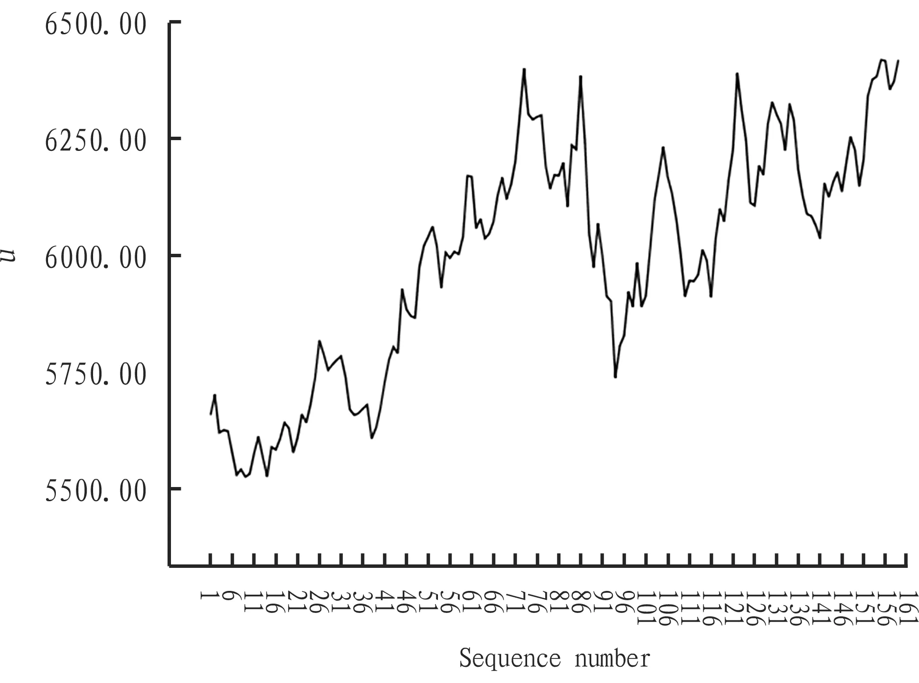
Fig.1Sequencediagramofu

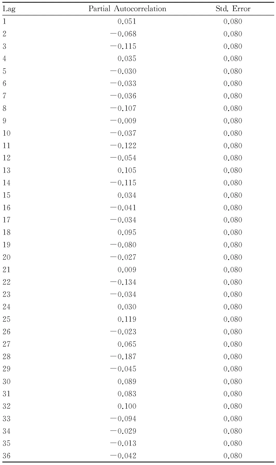
2.3.2Order of the autoregressive model (p). According to the calculation results of2.3.1, series is 1 order integration series. So, continue to calculate coefficient of partial autocorrelation faction of ut. Fig. 3 is drawn by the conclusion from Table 1. Fig. 3 shows the partial autocorrelation figure of ut series. In the autoregressive model, the 28th order is out of confidence interval. The coefficient is -0.187. So, the order of the autoregressive model is 28 (p=28).

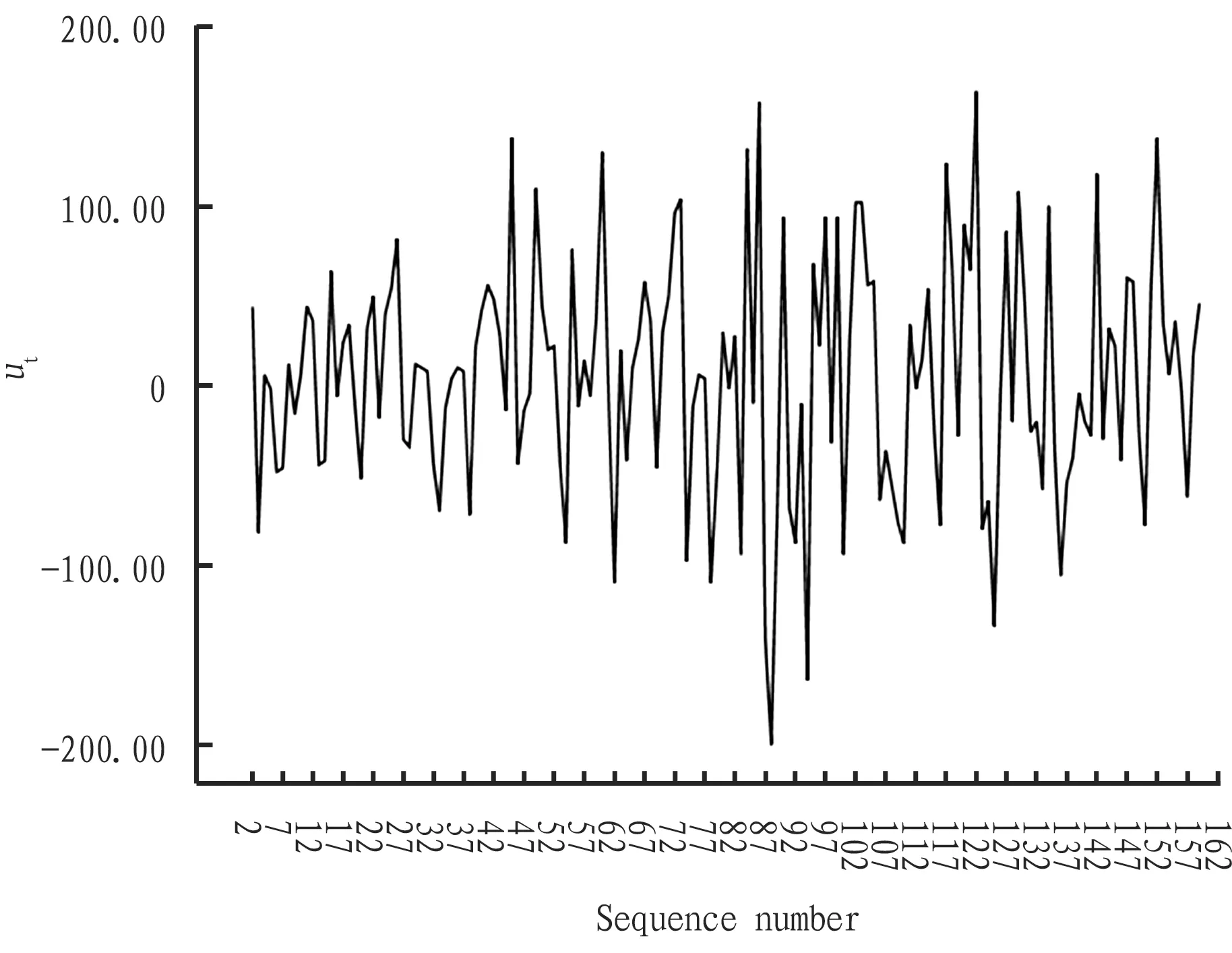
Fig.2Sequencediagramofut

Table1Partialautocorrelationofut

Series: u t

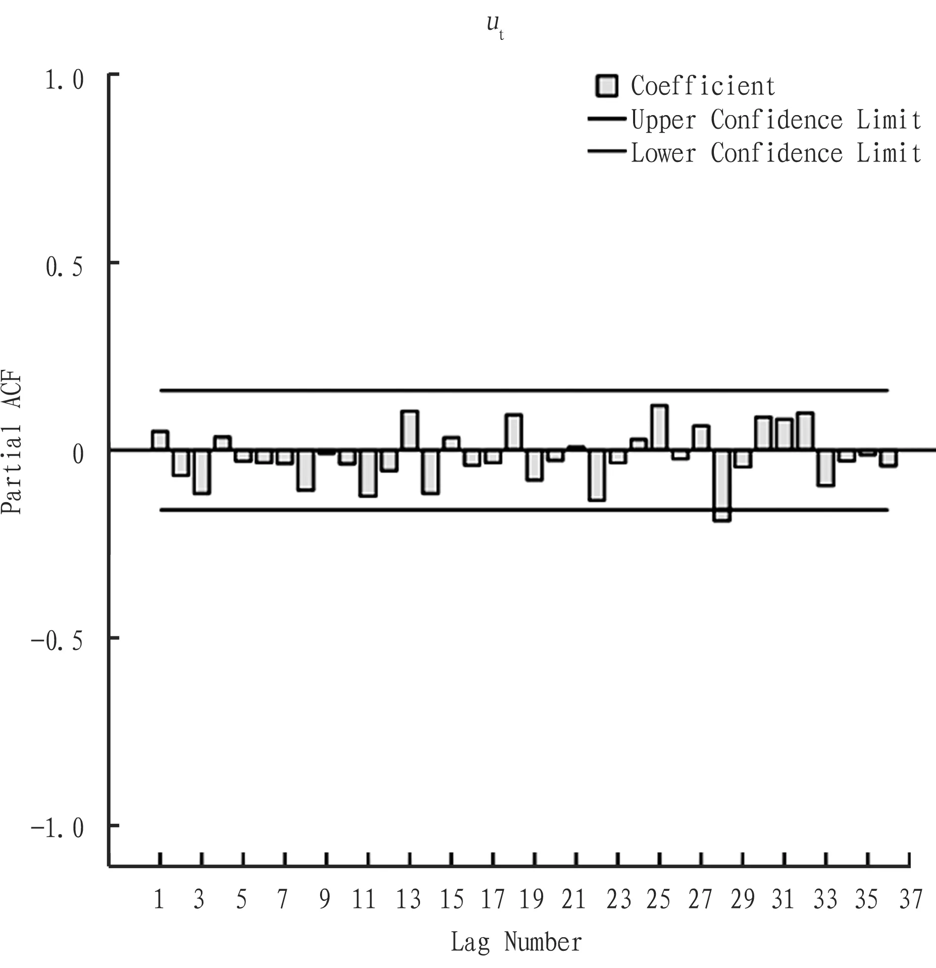
Fig.3Partialautocorrelationfactionofut

2.3.3Order of the moving average model (q). According to the calculation results of2.3.1, the autocorrelation coefficient ofutis shown in Table 2. Fig. 4 is drawn by the conclusions from Table 2. Fig. 4 shows the autocorrelation figure ofutseries. From Fig. 4, in the moving average model, the 25th order is out of confidence interval. The coefficient is 0.154. Therefore the order of the moving average model is 25 (q=25). The autocorrelation function is censored in the 25th order. The partial autocorrelation faction is censored in the 28th order, and ut series is 1 order integration series. Thus we establish ARIMA (28, 1, 25) model.

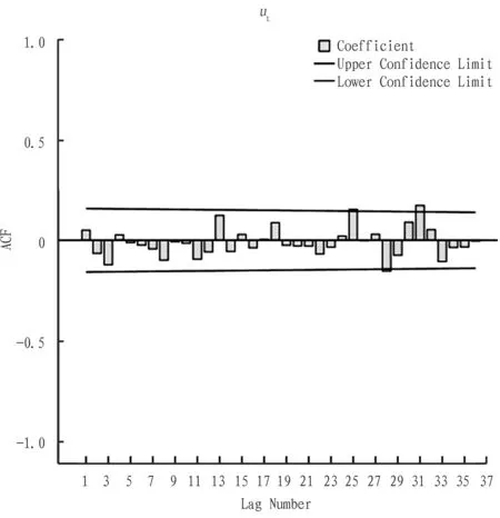
Fig.4Theautocorrelationfactionofut

2.4HypothesistestofresidualsAll lags of data in the confidence interval show that they are not obvious and not zero. From this conclusion, the residual of ARIMA (28, 1, 25) model of series has no serial correlation. This model passes the test, and it can be used in forecasting.

Table2AutocorrelationofutSeries:ut

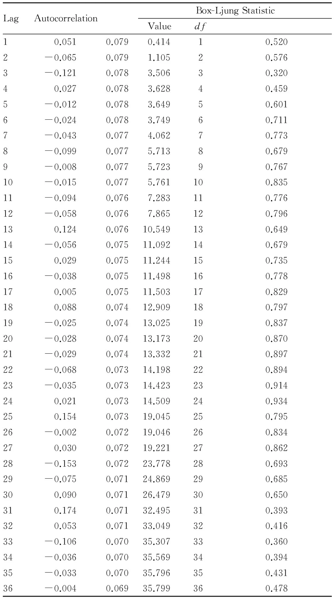
Note: The underlying process assumed is independent (white noise) based on the asymptotic chi-square approximation.

3 Application and discussion

3.1AccuracytestofforecastingThis paper uses ARIMA (28, 1, 25) model to fit the closing prices of soybean activity future contracts from January 4, 2016 to August 24, 2016, and draws the comparative line chart (see Fig. 6). From Fig. 6, we can see that this model highly fits the closing price of soybean oil active futures contract. Table 3 shows that determinant coefficientR-squared is 0.950, explaining many data. The data that can not be explained is only 0.05. And the value ofMAEandMAPEis 43.397 and 0.72, respectively. It shows that the model has few errors and good accuracy in application. Thus, ARIMA (28, 1, 25) model is feasible for short-term forecasting of futures.

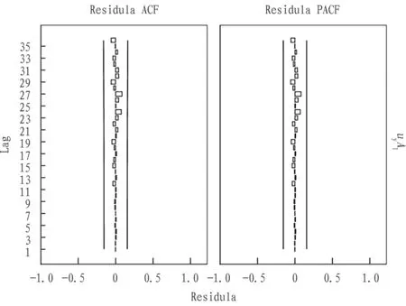
Fig.5ResidualcorrelationofARIMA(28,1,25)modelseries

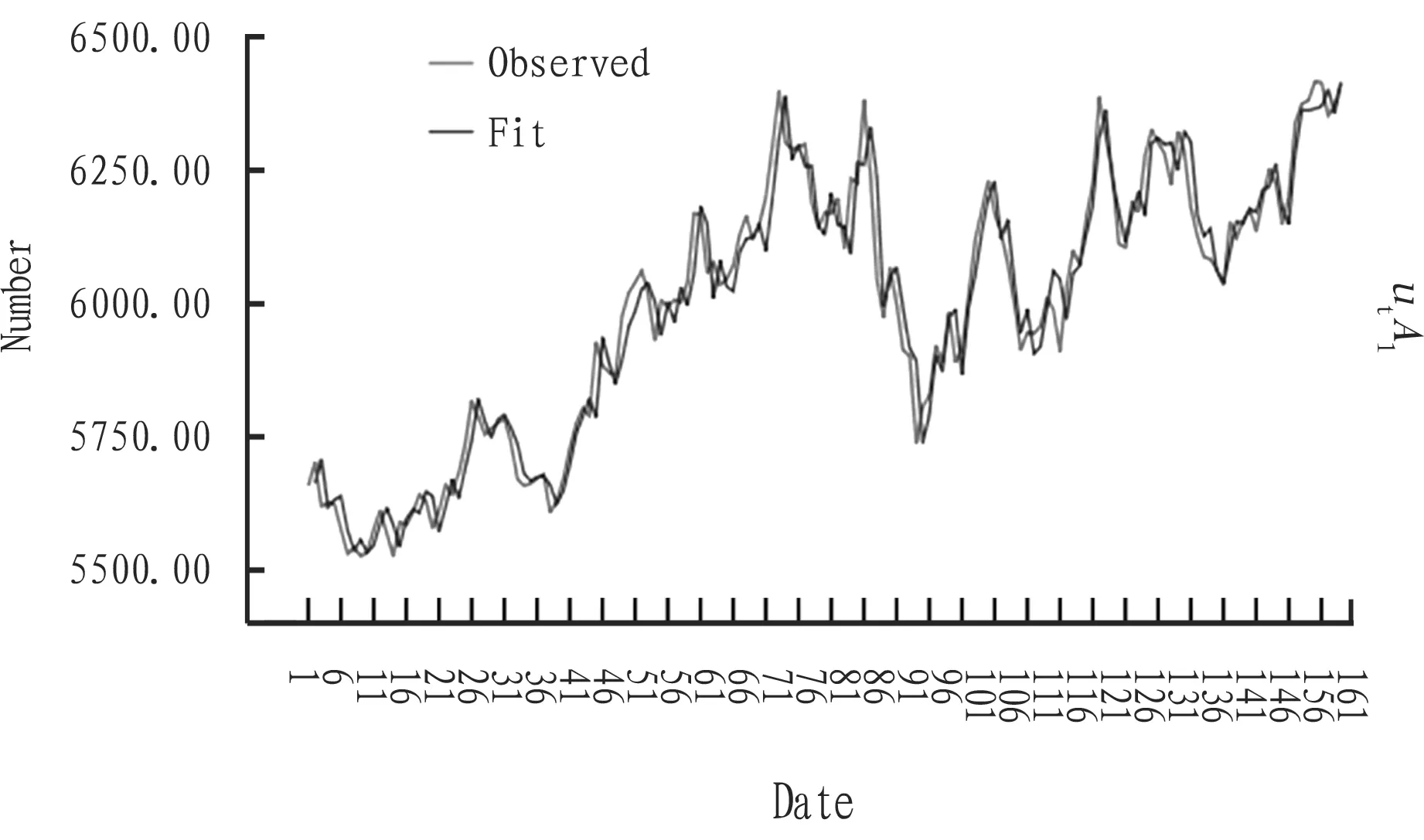
Fig.6Thefittingvalueandobservationvalueofuseries

3.2ForecastingofthepriceoffuturesWe use the established ARIMA (28, 1, 25) model to forecast series in next 30 lags. The results are shown in Table 4. Fig. 6 and Table 4 are combined together (Fig. 7).

Table3Modelfitting

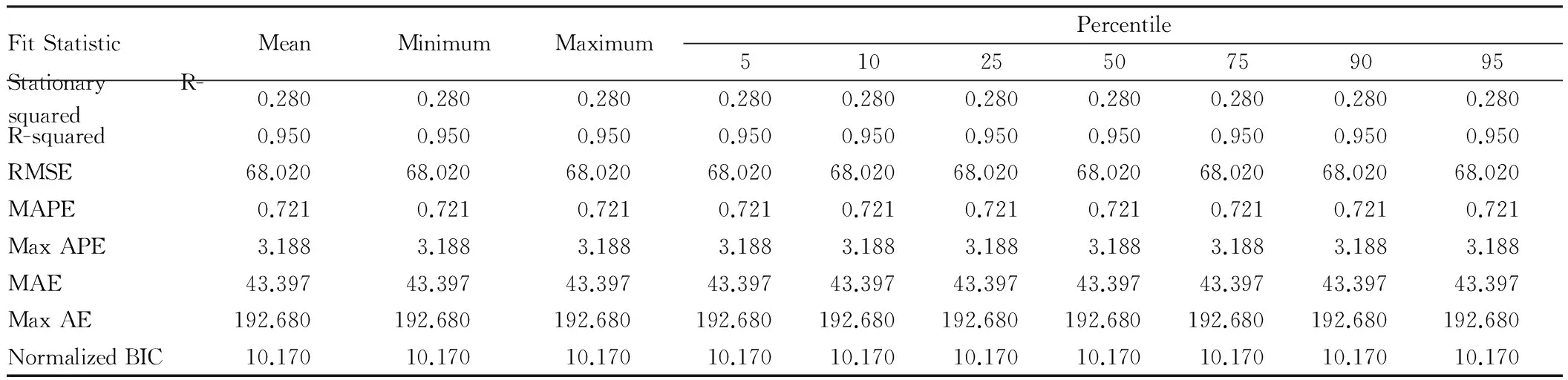
FitStatisticMeanMinimumMaximumPercentile5102550759095StationaryR-squared0.2800.2800.2800.2800.2800.2800.2800.2800.2800.280R-squared0.9500.9500.9500.9500.9500.9500.9500.9500.9500.950RMSE68.02068.02068.02068.02068.02068.02068.02068.02068.02068.020MAPE0.7210.7210.7210.7210.7210.7210.7210.7210.7210.721MaxAPE3.1883.1883.1883.1883.1883.1883.1883.1883.1883.188MAE43.39743.39743.39743.39743.39743.39743.39743.39743.39743.397MaxAE192.680192.680192.680192.680192.680192.680192.680192.680192.680192.680NormalizedBIC10.17010.17010.17010.17010.17010.17010.17010.17010.17010.170

Table4Forecastoftheclosingpriceofsoybeanoilactivefuturescontractinnext30tradingdays

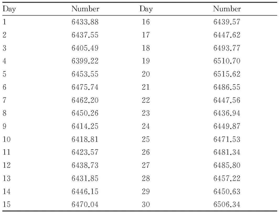
DayNumberDayNumber16433.88166439.5726437.55176447.6236405.49186493.7746399.22196510.7056453.55206515.6266475.74216486.5576462.20226447.5686450.26236436.9496414.25246449.87106418.81256471.53116423.57266481.34126438.73276485.80136431.85286457.22146446.15296450.63156470.04306506.34

4 Conclusions and discussions

The key to the forecast of the closing price of futures with ARIMA model is to use the historical closing price of futures ofTperiod to speculate on the futures price ofT+1 period. Now ARIMA model is widely used in a variety of areas for pricing prediction because of

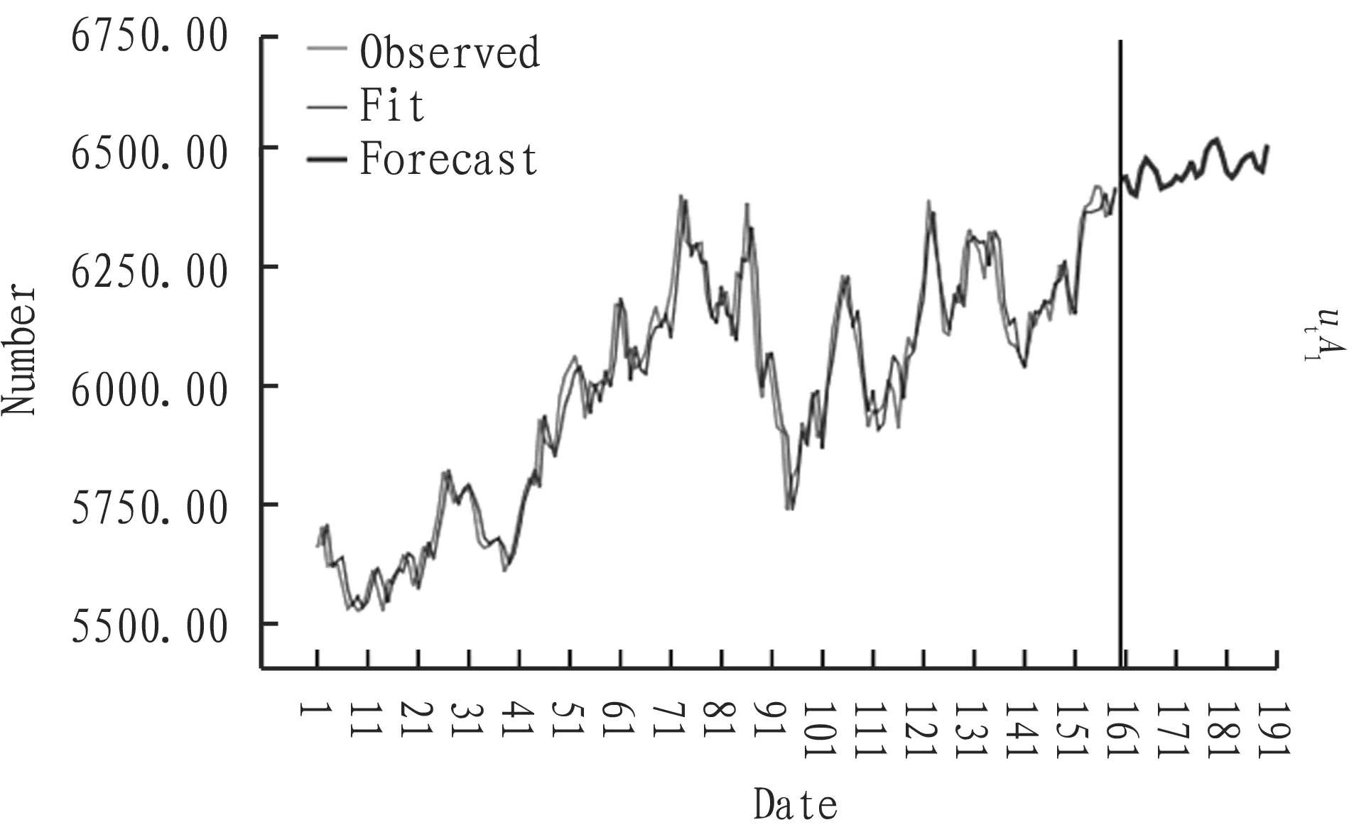
Fig.7Linechartofforecastingandhistoricaldata

its excellent ability of short-term forecasting. Whether the time series is non-stationary or stationary, both can be predicted by ARIMA. In general, the most economic series are non-stationary series. If we use ARIMA model to predict, the effect of trend does not matter and can be ignored. However, ARIMA model also has its deficiencies, that is, ARIMA model can only be used in short-term prediction. With increase in time, the variance of data will increase, and the error of prediction will also increase. As a result, there will be a large deviation between the predictive valueand the observed value. ARIMA model can not adjust uncertainty factors in the economic environment like good news in the market, market reaction to the news and the expectation of investors. Therefore, this model can only be used in short-term prediction, and it does not have good performance in long-term forecasting. In summary, although ARIMA model has shortcomings, it will acquire the precision data when it is used in short-term forecasting. This model provides an important method to predict price level of agricultural futures, and it will be of great significance to improving agricultural futures. This model can be used for the following aspects. First, it helps consumers to purchase agricultural products at lower price. This can reduce the non-necessary cost. The second one is that this model can show the arbitrage opportunities. Last but not least, it helps the investors who invest in futures market to receive the expected returns on investment, and it can make investors bear less loss in crisis or recession.

[1] XUE W. SPSS statistical analysis method and application [M]. Beijing: Publishing House of Electronics Industry, 2004: 402-474.

[2] NARENDRA B, PALLAVIRAM S. Partitioning and interpolation based hybrid ARIMA-ANN model for time series forecasting[J]. Sadhana, 2016, 41(7): 695-706.

[3] XU LP, LUO MZ. Short term analysis and prediction of gold price according to ARIMA model [J]. Finance & Economics, 2011(1): 26-34.

[4] ERNESTA G, EGLE B. Short-term wind speed forecasting using ARIMA model [J]. Energetika, 2016, 62(1/2): 45-55.

[5] PANG ZY, LIU L. If futures market can reduce the volatility of agricultural price by Discrete wavelet transform and GARCH model[J]. Journal of Financial Research, 2013 (11): 130-143.

[6] LIU F, WANG RJ, LI CX. Application of ARIMA model in forecasting agricultural product price [J]. Computer Engineering and Applications, 2009, 45(25): 238-239.

[7] CHI QS. Analysis of the growth trend of China’s oil consumption base on ARIMA model [J]. Resources Science, 2007, 29(5): 69-73.

[8] XIONG Y, SUN YD. The factors that affect the price of soybean futures in China [J]. Journal of South-Central University, 2004, 23(2): 100-102.