An Error Estimator for the Finite Element Approximation of Plane and Cylindrical Acoustic Waves.

J.E.Sebold,L.A.Lacerdaand J.A.M.Carrer

An Error Estimator for the Finite Element Approximation of Plane and Cylindrical Acoustic Waves.

J.E.Sebold1,L.A.Lacerda2and J.A.M.Carrer3

This paper deals with a Finite Element Method(FEM)for the approximationof the Helmholtz equation for two dimensional problems. The acoustic boundary conditions are weakly posed andan auxiliary problem with homogeneous boundary conditions is defined.This auxiliary approach allows for the formulation of a general solution method.Second order finite elements are used along with a discretization parameter based on the fixed wave vector and the imposed error tolerance.An explicit formula is defined for the mesh size control parameter based on Padé approximant.A parametric analysis is conducted to validate the rectangular finite element approach and the mesh control parameter.The results of the examples show that the discrete dispersion relation(DDR)can be used for the rectangular finite element mesh refinement under predefined error tolerances.It is also shown that the numerical formulation is robust and can be extended to higher order finite element analyses.

Numerical Methods in Engineering,Finite Element Method,Helmholtz Equations,Plane and Cylindrical Wave Propagation.

1 Introduction

Numerical solutions of the Helmholtz Equation are well-known in literature,where finite and boundary element methods of aproximation have been proposed for a broad range of problems.

One particular issue addressed by many authors is the necessary/minimum mesh discretization for the solution approximation for a fixed wavenumber.See for instance,Harari et al.(1996),who used the technique of dispersion analysis to include complex wavenumbers.In addition,complex Fourier analysis techniques wereused by them to observe the dispersion and attenuation characteristics of thepversion finite element method.Based on numerical evidences they conjectured that the elements of degreepprovide an approximation of order 2pfor the dispersion relation in the limit when the element size tends to zero. Ainsworth(2003)analyzed the discrete dispersion in the aproximation by finite elements with relatively high wavenumbers.Sarkar et al.(2011)showed that in finite flexible structural acoustic waveguides have a general form for the dispersion equation.Christon(1999)considered the dispersive behaviour of a variety of second order finite elements for wave equations and presented numerical comparisons between the discrete phase,group velocity and the analytical value.Babuška et al.(1995)studied the scattering properties of high order finite elements for the Helmholtz equation in one dimension,and obtained estimates up to the fifth order approximation,in which the product between the temporal frequency and the mesh parameter is smaller than one,that is,whenωh＜1.The same article presents numerical evidences,which lead to the conjecture that elements of orderphave an order approximation 2pfor dispersion relation when the mesh parameterhtends to zero.Sebold et al.(2014)presented analytical expressions that provide information to the mesh control of edge finite element for the approximation of Maxwell’s equations.Such expressions were generated from the numerical phase velocity and dispersion analysis.Another important task in the present work is the use of hierarchical basis functions,Adjerid(2002).A hierarchical basis has the property that the base levelp+1 is obtained by adding new functions to the base levelp,i.e.,the base as a whole does not need to be rebuilt when the degree of the polynomial is increased.This property is desirable,if not essential,when using thep-version of the finite element method.The hierarchical basis functions in one-dimension are defined as integrals of Legendre polynomials.Thus,the orthogonality properties are guaranteed,leading to sparse and well conditioned stiffness matrices.Although the proposal of analytical expressions for the mesh refinement,based on the discrete dispersion relation,is a significant contribution of this article,the main novelty is the presentation of a contribution applied to acoustic which related with the works mentioned above.This contribution enables one to extend the work of Sebold et al.(2014)to nodal finite elements,unifying,from this point of view,the acoustic studies presented by Christon(1999)for numerical phase velocity and Babuška et al.(1995)for discrete dispersion relation.

In this study the discrete dispersion relation suggests the used of the phase velocity number as an error estimator for the finite element approximation of the Helmholtz equation.The analytical expressions for the numerical phase velocity can be used to estimate the approximation error in the presence of plane or cylindrical waves,thus providing a faster,more efficient and less expensive computationally way to obtain results within an imposed error margin.It is the authors’reasoning that restricting the study to quadrilateral elements is a convenient way to provide an initial understanding for those readers interested in the foundations of this theory.

2 Basis functions

Let Ω be an open and bounded domain in the real set R,and letbe a subspace of piecewise continuous polynomials of degreep∈Z+withmvariables denoted by

whereC0(Ω)is the space of all continous functions on Ω,H1(Ω)is the Hilbert space of differentiable functionsu,such thatuandwithj=1,...m,are integrable square functions.

2.1 Legendre hierarchical base functions

LetMjbe the set of Legendre polynomials de fined on a reference element Ωe,which are given by Rodrigues formula,Olver et al.(2010),for 0≤j≤pas:

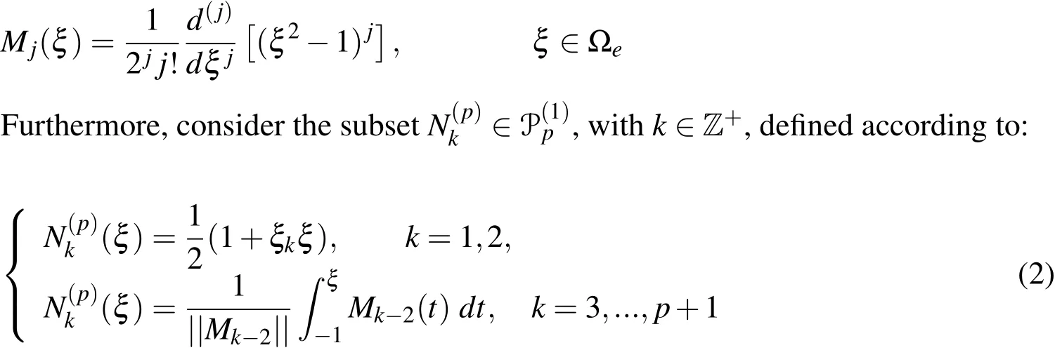
The functions de fined by equations(2)form what is called Legendre Hierarchical Shape Functions,Harari et al.(1996)and Thompson and Pinsky(1994).

2.2 Hierarchical base functions for rectangular elements of p-order

whereXp,qis the monomial set of degree less or equal topinξand of degree less or equal toqinη,i.e.

Thus,the basis functions with two variables,ξandη,of orderp=q,are given by the tensor product

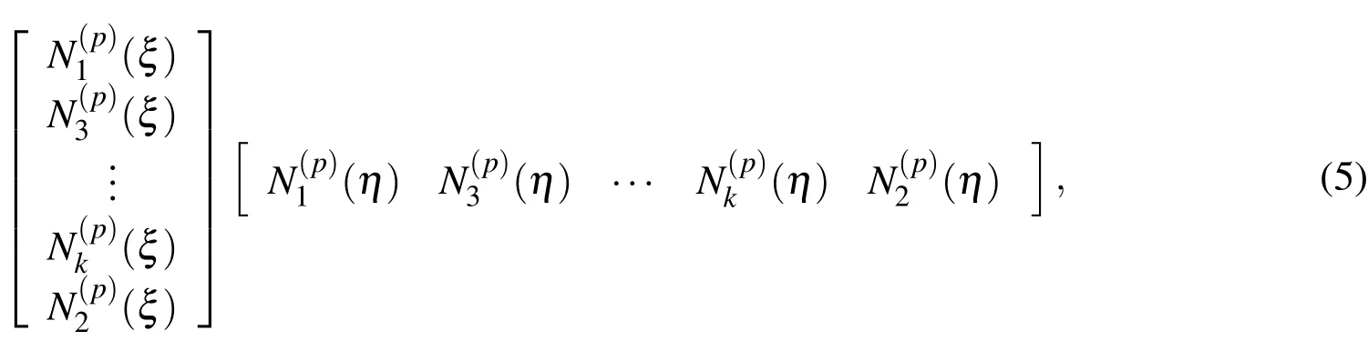
Thus,it follows that each basis functionand withi,j=1,2,3,associated with the nodel,appears at the tensor product entries,see equation(6)and Figure 1(a),

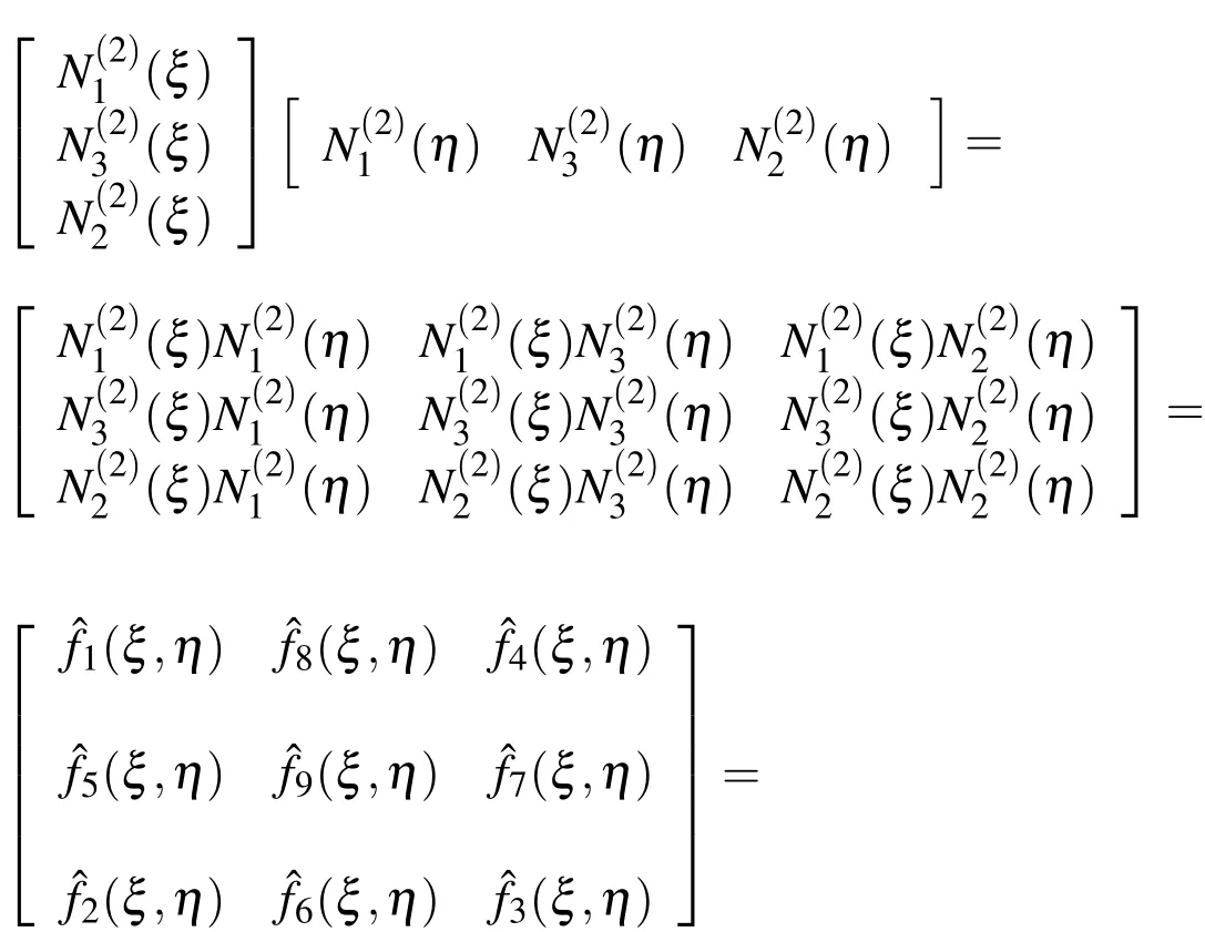
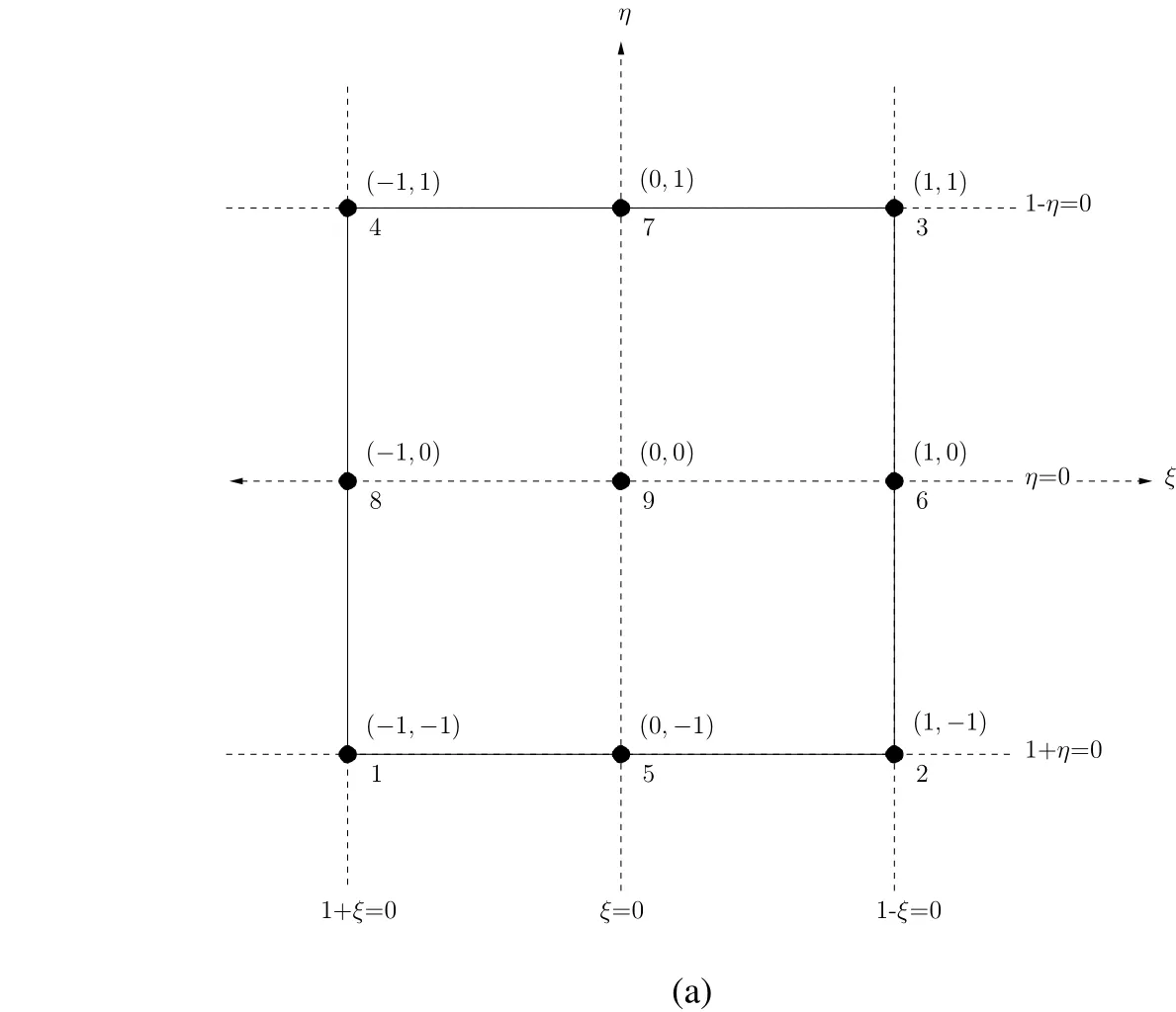
Figure 1:Reference element Ωeassociated with the basis functions of p=2.

3 Helmholtz equation and the finite element method approach

3.1 Plane wave

Let Ω ⊂ R2be a domain with boundary Γ.The homogeneous acoustic wave equation can be written as

For time harmonic waves,a solution of equation(7)can be written as

Furthermore,one can assume that the wave vector κ =(κ1,κ2)is related to the circular frequency ω by the dispersion relation,Oliveira et al.(2007),

Thus,the following variational problem,present in Liu(2009),can be stated:Find∈H1such that

in which(·,·)L2denotes the inner product L2(Ω).The problem(11)is subject to boundary conditions

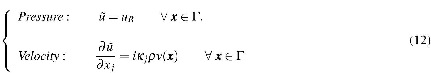
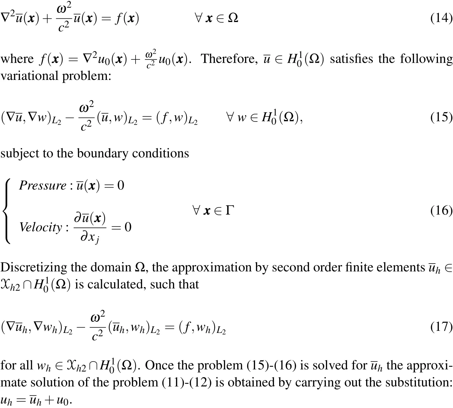
An alternative approach,which aims a simpler programming solution for the problem(11)-(12),is presented in the sequence.The idea is to establish,from u( xxx)data,a new problem with homogeneous boundary conditions. The new problem is solved with second order finite element method using the Legendre hierarchical shape functions for retangular elements.Once the solution to the new problem has been found,the next step is the recovery of the solution of the problem given by equations(11)-(12).For this approach,is de fined,as well asThus,one has the new boundary conditions:j=1,2.Proceeding this way,the problem de fined by(11)-(12)turns into the nonhomogeouos problems

3.2 Cylindrical wave

Another relevant case appears when one has as solution of(14)the convolution

where g,f∈Lp(Ω),with 1≤ p≤∞,has compact support in the domain Ω⊂Rd,with d=1,2,...,n.In the solution(18),g is known as free space Helmholtz Green’s function,Beylkin et al.(2009).Furthermore,the function g satisfy

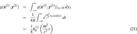
The main interest of this work is the case d=2.Thus,the fundamental solution in two dimensions can be obtained by takingand the identity cosh(θ)−sinh(θ)=1 for any θ angle.Thus,by taking

Suppose the cylindrical waves expanding from a punctual source which is located at(0,0)∈R2,see Figure 2(a).Finite element approximation is considered on square domain Ω⊂R2extracted from Figure 2(a)(see Figure 2(b)).

3.3 Numerical experiments

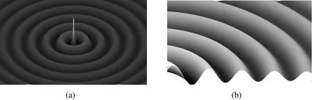
Figure 2:(a)Cylindrical wave;(b)Domain Ω.

Figure 3(a)shows the analytical solution of the problem(11)-(12),while Figure 3(b)shows the result of alternative approach suggested using second order finite elements,the wave vector κ =(10π,10π),h=1/16 and the Legendre hierarchical basis functions for rectangular elements.Figures 4(a)and 4(b)show the exact solution(21)and finite element approach,respectively,referring to the cylindrical wave.This approximation is calculated using the same wave vector and the same parameterhfor the plane wave approximation.

Figures 5(a),5(b)and 5(c)depict the diagonal slice in the(1,1)direction of the plane wave from Figure 3(a),and of the discrete surface encountered by alternative approach from Figure 3(b),at different levels of re finement:h=1/16,h=1/32,h=1/64.

Figures 6(a),6(b)and 6(c)depict the diagonal slice in the(1,1)direction of the region propagation Ω =[1,1]×[2,2]of the cylindrical wave,Figure 4(a),and of the discrete surface encountered by alternative approach,Figure 4(b),at different levels of re finement:h=1/16,h=1/32,h=1/64.

Figure 3:(a)Analytic solution of the problem(11)-(12);(b)Alternative finite element method approach with p=2,κ =10π and re finement level h=1/16.

Figure 4:(a)Analytic Solution for cylindrical wave;(b)Alternative finite element method approach for cylindrical wave with re finement level h=1/16.

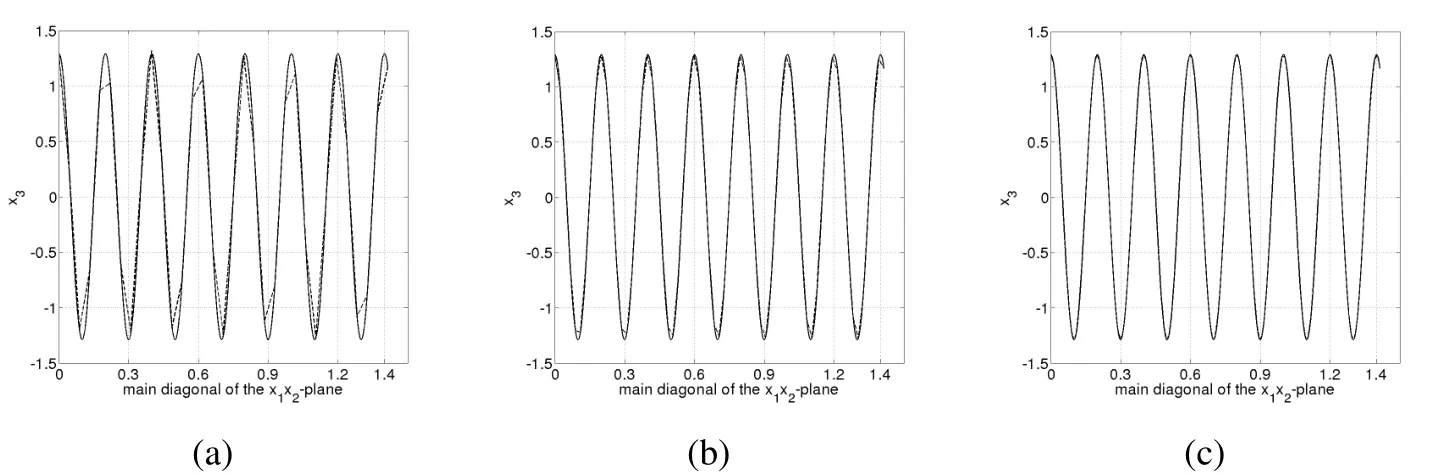
Figure 5:(a),(b)and(c)depict the diagonal slice in the(1,1)direction of the plane wave,at different levels of re finement,h=1/16,h=1/32,h=1/64,respectively.

Figure 6: (a),(b)and(c)depict the diagonal slice in the(1,1)direction of the region propagation Ω =[1,1]× [2,2]of the cylindrical wave,at different levels of refinement,h=1/16,h=1/32,h=1/64,respectively.

4 Discrete dispersion relation

First let’s establish some requirements for the definition of the discrete dispersion relation for the scalar Helmholtz equation in two dimensions must be establish.Suppose that a uniform mesh sizewith n∈Z,is placed on the real line with nodes located at hZ,where Z is the set of integers.The set of continuous piecewice linear functions on the mesh is denoted Xh1.In analogy to the continuous problem de fined by equation(7),one should be concerned with solutions of the form

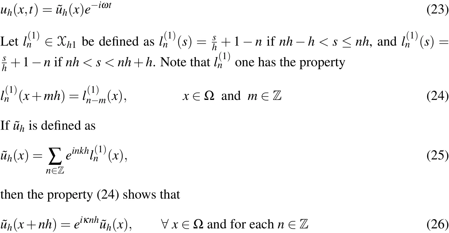
Thus,the analysis can be performed uniformly at any point of the mesh.The function∈Xh1is a discrete version of the complex exponential(s)=eiκs,where κ is the wavenumber,which is related to the frequency ω by the dispersion relation,found at Oliveira et al.(2007),and written below

Considering the Helmholtz equation in one dimension

the following variational problem can be stated:Find∈Xh1such that

From another point of view,one can consider(29)as an eigenvalue problem,where ωh(κ)2can be calculated by settingIn fact,after replacing equation(25)

into equation(29)and noting thatfollowing a similar statement forthen follows

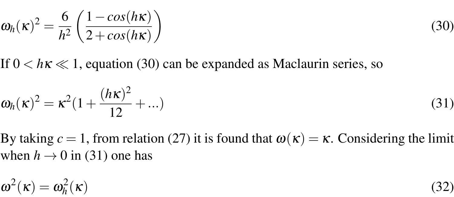
Expression(32)corresponds to the discrete dispersion relation for the scalar Helmholtz equation in one dimension.

4.1 Discrete dispersion relation for the Helmholtz equation in two dimensions

Suppose now that we have a real plane with nodes located at hZ2.The set of continuous piecewice polinomials with degree p less than or equal to two on the mesh is denoted Xh2.In analogy to the solution of the continuous problem de fined by equation(25),one should be concerned with solutions of the form

Replacing(36),(37)and(38)in(35)the discrete dispersion relation for the Helmholtz equation in two dimensions is obtaind.It is written as follows:

4.2 Discrete dispersion relation for elements of p-order.

In order to use equation(30),it is desirable to expressωh(κ)in terms ofκ.A practical way to achieve this goal consist is finding an implicit de finition forωh(κ)in terms ofcos(hκ).For example,for the case of elements of the first order,relation(30)can be rewritten as

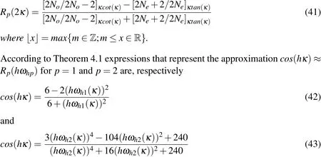
Teorema 4.1Let[2Ne+2/2Ne]κtan(κ)and let[2No/2No−2]κcot(κ)be the notations for the Pad approximation of κtan(κ)and κcot(κ),respectively,where Ne=Thus,ωhpsatis fies cos(hκ)≈Rp(hωhp),where Rpis a rational function

5 Parameter selection for mesh

Now the theory developed in the two previous sections is used to establish a criterion for selection of the mesh refinement parameter n for second order rectangular elements.

First,consider the speed of numerical phase as

Second,to establish a connection with the numerical experiments carried out in Section 3,consider a wave vector with the same characteristics as that used in the approximation of the problem(11)-(12),i.e., κ =(κ,κ).Thus,note that ω2=2κ2C2.On the other hand,equation(39)shows that ω2=2ωh(κ)2,consequently

Considering the cos(hκ)approximations for p=1 and p=2,equations(42)and(43),respectively,the numerical phase velocity C can be written as a function of hκ,thus obtaining,

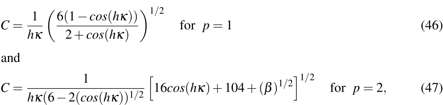
where β =(16cos(hκ)+104)2−960(cos(hκ)−3)(cos(hκ)−1).

However,from dispersion relation(10)of the continuous problem,the exact phase velocity is given by c=1.For example,for p=2,Figure 7(a)shows the exact phase velocity compared with the numerical phase velocity given by equation(47).Figure 7(b)presents a closer view of Figure 7(a),with 0≤hκ≤1,from which it is possible to determine,for example,the minimum value of the parameter h so that the estimated phase velocity error is less than 0.01%.This is done simply by observing the point at which the velocity curve reaches the value 1.0001(or hκ≈0.62).

Note that the wave vector in the numerical example was κ =10π(1,1),then by taking κ =10π,has h ≈Consequently,for n≥51,the error between the approximated and exact phase velocity is less than 0.01%.The possible use of this approximation for mesh refinement is now evaluated through a convergence analysis.

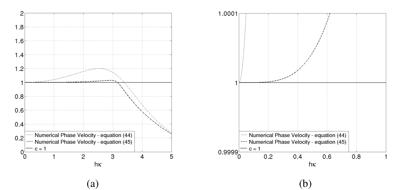
Figure 7: (a)Numerical phase velocity for first and second order elements;(b)Closer view of Figure 7(a).

5.1 Convergence analysis

Letdbe the relative error in the phase velocity given by|1−C|.Equation(46)is employed to show the phase velocity approximation for a fixedκand an increasingn.This is shown in Figure 8(a)for three differentκvalues and,as expected,it is clear that improving the approximation forcrequires smallerhvalues for larger frequency numbers.For convenience,it would be interesting to vali-date the equation(27)for problems in two dimensions.To do so,it is assumed that κ=κ(cos(θ),sin(θ)).Letua∈H1(Ω)bedefinedbyNote que uais an analytical solution of problem(11)-(12).

观察组患者采取ACEI药物治疗，10 mg/d的苯那普利，对于高血压患者降压效果不好可加至20 mg/d，对照组患者采取非ACEI药物治疗，使用钙离子拮抗剂、β受体阻断剂等。两组患者治疗时间均为3个月。

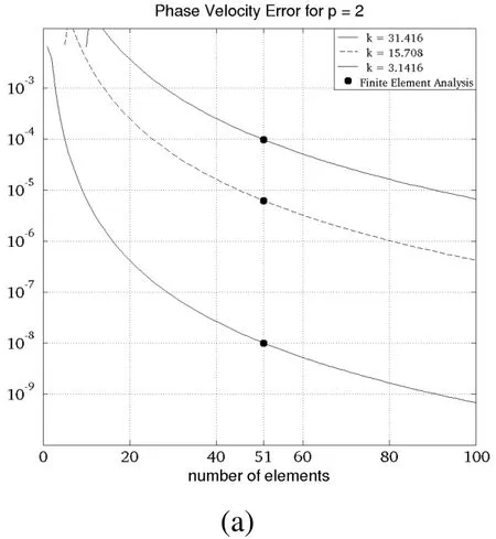
Figure 8:Phase Velocity approximation by Equation(47)with increasing discretization and FEM results for n=51.

For calculation purposes let||·||be the norm for a real value function,de fined by

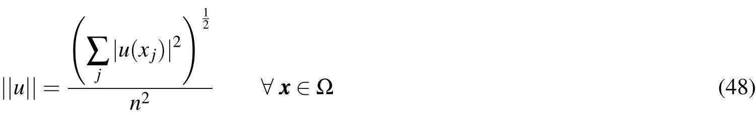
Consideruh∈Xh2the Finite Element numerical solution of problem(11)-(12),with 51 elements in the mesh discretization.By taking the same direction of propagation of the plane wave of the numerical experiment,i.e.,one can de fine uadj∈H1by

that are analytics solutions within the range 0.9＜cadj＜1.1.Furthermore,we consider the analytical solutions of diagonal points of the domain Ω,i.e.,x1=x2,are considered.The error norm||uadj−uh||is shown in Figure 9(a),where can be noticed that the numerical result is better adjusted by an analytic expression with cadjvery close to 1.A closer view is shown in Figure 9(b)where it becomes clear that the numerical phase velocity error is in neighborhood d＜0.01%,conforming the estimated result obtained from 7(b).

Figure 9:(a)Error norm with 51 elements in the mesh indicating the better adjust by analytic expression with cadjvery close to 1;(b)Closer view of Figure 9(a).

The same analysis can be made for the experiment involving cylindrical waves.In this version,uadjis de fined according to:

whereris the distance between any point on the diagonal of the domain Ω=[1,1]×[2,2]and the point(0,0).Figures 10(a)and 10(b)show the error norm reaching its lowest value,≈10−7,also in the neighborhoodd＜0.01%ofcadj≈1.

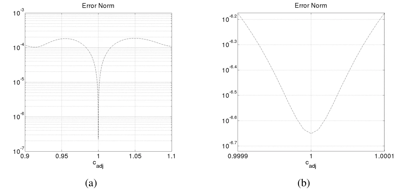
Figure 10:(a)Error norm with 51 elements in the mesh indicating the better adjust by analytic expression with cadjvery close to 1;(b)Closer view of Figure 10(a).

In both experiments,with plane and cylindrical waves,the correlation between the error in the numerical phase velocity and the error of the approximation by finite element is evident and shows that the phase velocity equations obtained from the discrete dispersion analysis may be used as error estimators in the FEM solution of the Helmhotz equation problems.

6 Conclusion

The use of Legendre hierarchical basis functions facilitate the computer implementation of the finite element method for solving Helmholtz equation problems.It is always possible to take advantage of the functions used in the approximation of order p in the numerical experiments of orderp+1.Solution approximations of a simple numerical problem with fixed wavenumber were presented,until fourth order,demonstrating the already known efficiency of the method.

From the variational formulation of the Helmholtz equation the already known expression of the discrete dispersion relation was presented for a finite element space of orderp=1.Such relation was reformulated with aid of Padé approximation and extended to spaces of elements of orderp=2.A direct link between the phase velocity,written as a function of the discrete dispersion relation,and the size of the elements used in domain discretization is shown for ordersp=1 andp=2.Graphical interpretation of these equations clearly indicate the phase velocity error reduction with the increasing mesh refinement for several wavenumbers.

Finite element analyses were carried out and con firmed the validity of the developed phase velocity equations forp=1 andp=2.FEM results were fitted to obtain a numerical phase velocity and it was shown that the best fit was in perfect agreement with the error estimates derived from the phase velocity equation and the number of elements in the uniform discretization.

Error norms were evaluated in all FEM analysis and a strong correlation was observed with the phase velocity error in the analyzed problem.This evidence suggests that the numerical phase velocity de fined from the discrete dispersion can be used as an error estimator in the approximation of the Helmholtz equation by the finite element method.

Adjerid,S.(2002):Hierarchical finite element bases for triangular and tetrahedral elements.Comput.Methods Appl.Mech.Engrg.,vol.190,pp.2925–2941.

Ainsworth,M.(2003):Discrete dispersion for hp-version finite element approximation at high wavenumber.SIAM J.Numer.Analysis,vol.42,pp.553–575.

Babuška,I.et al.(1995): Dispersion analysis and error estimation of Galerkin finite element methods for the Helmholtz equation.International Journal for Numerical Methods in Engineering,vol.38,pp.3745–3774.

Beylkin,G.et al.(2009):Fast convolution with the free space Helmholtz Green’s function.Journal of Computational Physics,vol.228,pp.2770–2791.

Christon,M.(1999):The influence of the mass Matrix on the dispersive nature of the semi-discrete,second-order wave equation.Methods Appl.Mech.Engrg.,vol.173,pp.146–166.

Harari,I.et al.(1996): Recent Developments in Finite Element Methods for Structural Acoustic.Archives of Computational Methods in Engineering,vol.36,pp.131–311.

Liu,Y.(2009):Fast Multipole Boundary Element Method.Cambridge University Press.

Monk,P.(2003):Finite Element Methods for Maxwell’s Equations.Oxford Science Publications,New York.

Oliveira,S.P.et al.(2007): Optimal blended spectral-element operators for acoustic wave modeling.Geophysics,vol.72,no.5,pp.95–106.

Olver,F.et al.(2010):NIST-Handbook of mathematical functions.Cambridge University Press,New York.

Sarkar,A.et al.(2011):Unified Dispersion Characteristics of Structural Acoustic Waveguides.Computer Modeling in Engineering&Sciences,vol.81,no.3,pp.249–268.

Sebold,J.E.et al.(2014): Construction of an edge finite element space and a contribution to the mesh selection in the approximation of the second order time harmonic Maxwell system.Computer Modeling in Engineering&Sciences,vol.103,no.2,pp.111–137.

Thompson,L.;Pinsky,P.(1994):Complex wavenumber Fourier analysis of the p-version finite element method.Computat.Mech.,vol.13,pp.255–275.

1Federal Institute of Education,Science and Technology-Campus Araquari,Santa Catarina,Brazil

2Institute of Technology for Development,Curitiba,Paraná,Brazil.

3Federal University of Paraná,Curitiba,Paraná,Brazil.