The impact of macroalgae on mean and turbulent flow fields*

THOMAS Robert E., MCLELLAND Stuart J.

Department of Geography, Environment and Earth Sciences, University of Hull, Hull, UK, E-mail: r.e.thomas02@members.leeds.ac.uk

The impact of macroalgae on mean and turbulent flow fields*

THOMAS Robert E., MCLELLAND Stuart J.

Department of Geography, Environment and Earth Sciences, University of Hull, Hull, UK, E-mail: r.e.thomas02@members.leeds.ac.uk

(Received December 25, 2014, Revised March 15, 2015)

In this paper, we attempt to quantify the mean and turbulent flow fields around live macroalgae within a tidal inlet in Norway. Two Laminaria digitata specimens ～0.50 mapart were selected for detailed study and a profiling ADV was used to collect 45 velocity profiles, each composed of up to seven 0.035 m-high profiles collected for 240 s at 100 Hz, at a streamwise spacing of 0.25 m and cross-stream spacing of 0.20 m. To quantify the impact of the macroalgae, measurements were repeated over a sparser grid after the region had been completely cleared of algae and major roughness elements.

dealiasing, laminaria digitata, turbulence, vectrino profiler, velocity profile

Introduction

In recent years, a significant amount of research has examined the interactions between immersed vegetation and flowing water[1,2]. Whilst early physical modeling and theoretical studies employed rigid structures such as wooden dowels, recent studies have progressed to flexible surrogate plants[3-8]. However, even appropriately-scaled flexible surrogates fail to capture the variability in thallus morphology, flexibility and strength, both within and between individuals[9], and frontal area (for rigid organisms) or planform area (for flexible organisms like macroalgae[10]) over space and time[11]that may force spatio-temporal variability in mean and turbulent flow fields[7]. For example, in their flume experiments, Siniscalchi and Nikora[12]found that different species of aquatic plants responded differently to similar hydrodynamic forcing.

Aquatic vegetation can form dense, uninterrupted canopies as well as distributed patches. There have been a number of experimental and computational studies on the mean fully-developed flow and turbulence characteristics through and over large, uniform stands of vegetation[3,6,13-16]. However, macrophyte growth in rivers and macroalgae colonization of coastlines is typically patchy and, therefore, Naden et al.[17]appealed for experimental work to improve understanding of the effect of vegetation patches or individual large plants and their arrangement on flow fields. Experimental studies suggest that the extent to which a patch modifies the flow field is dependent upon the frontal or planform area. Zong and Nepf[18]reported that the effect of a dense patch is equivalent to a solid body of the same width, streamwise velocity begins to decrease approximately one patch width upstream of the patch. Conversely, turbulence levels increase at the leading edge of a patch[18]. As the frontal or planform area tends to zero, the adjustment length also tends to zero. Velocity is strongly reduced within a patch, whereas the flow is highly accelerated above and around it[17]. However, at low-speed flows, a zone of increased velocity occurs near the bed that extends along the length of the patch[8]. Velocities tend to be laterally uniform over most of the patch width, increasing toward the free stream within a few stem diameters of the patch edge[18]. A horizontal shear layer with a width comparable to the patch width[19]develops between the water-surface and a specific depth within the canopy[4], while a near-vertical shear layer may also form at the patch edge[20]. Coherent vortices in these shear layers may dominate the turbulent flux of momentum across the patch edge[20], but the threedimensionality of the wake and high background turbulence levels should disrupt periodic vortex formation[21]. At the downstream edge of a patch, velocityprofiles slowly return to the undisturbed upstream condition. Folkard[5]studied the effects of the wake caused by one patch on an adjacent downstream patch and found that patch spacing relative to total wake length and the location of the wake Reynolds stress maximum controlled the turbulence within the downstream patch. Wake length was a function of discharge, leaf length, flow depth, and patch separation[5]. Maltese et al.[7]focused on the spatial patterns of coherent turbulent structures in vegetation gap environments.

Although a number of field studies have been carried out[17,19,21,22], measurements of hydraulic variables have generally been limited to time-averaged ata-point measurements that aim to approximate the depth-mean velocity. This is problematic because in spatially heterogeneous flows, point measurements are dependent upon the sampling location[23,24]. For example, measurements over entire channel cross-sections[17,19]indicated that velocity profiles are highly variable and dependent on the locations of plants and the type of plant assemblage. Fairbanks and Diplas[4]examined turbulence statistics in the vicinity of a rigid canopy and found that both the longitudinal and vertical turbulence intensity profiles were variable and dependent on the spatial sampling location. Such sensitivity may be ameliorated through application of the double averaging methodology over an appropriate spatial averaging volume[23,24].

Thus, there is a need to undertake experimental work using live plants, in order to quantify the mean and turbulent flow fields within and around different plant forms under different flow velocities and depths, especially in natural environments[17]. Furthermore, although marine macroalgae tend to have morphologies that are significantly different to those of freshwater macrophytes, no studies have sampled the flow patterns and turbulence characteristics around macroalgae and their impact upon flow fields has thus not been quantified. In the present study, we therefore quantify: (1) the mean and turbulent flow fields around macroalgae at a vegetated field site, (2) the locations and biomechanical properties of the algae[25], and (3) the mean and turbulent flow fields after algae were completely removed.

1. Methods

The study site is a small tidal inlet located at the entrance of Trondheimsfjord, Sør-Trøndelag, Norway (see Figs.1 and 2). The inlet is approximately triangular in planform, with its mouth to the northwest. The deepest parts of the inlet are to the centre and northeast, where the depth is between 25 m and 30 m. A delta, formed of coarse sand and broken shells, has been deposited in the northwest corner of the inlet (Fig.2). This delta is fed by a channel with a gravelcobble bed that is 15 m wide and up to 4 m deep at the bridge that marks the seaward margin of the inlet (Fig.2). This outlet channel is pinned to the northern edge of the delta and thus the depth of water over the delta shallows from west to east and from north to south. For much of the delta, the average water depth above the flat sandy bed is ～0.5 m.

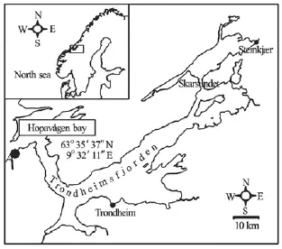
Fig.1 Location of the study area in Norway

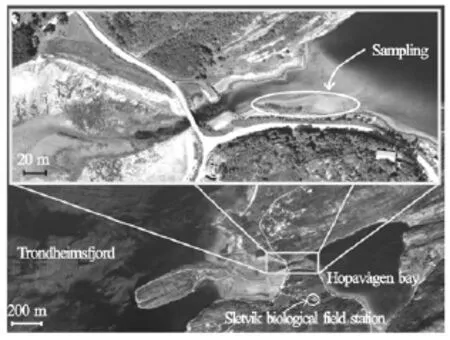
Fig.2 Aerial photographs of the study area (fromwww. norgeskart.no)

An 11 m long×6 m wide region in the southwestern part of the delta was selected for intensiv2e study. Due to the dimensions of the inlet (370 000 m) and the small cross-sectional area of the outlet channel, the tidal range is relatively small, during the sampling period (May 2012), the water level in the study area varied by ～0.5 m. Tides are semi-diurnal, strongly asymmetric and flood-dominated, the flood tide lasts for～3.5 hwhile the ebb lasts for ～8.5 h. All velocity measurements were made during the ebb tid2e. The catchment area of the bay is negligible (1.9 km). Therefore, the salinity in the inlet is close to the values found in the fjord(31±4 ppm), and varies depending on the thermal and tidal conditions. Within the 11 m×6 m region, two Laminaria digitata specimens～0.50 mapart were selected for detailed study and a 2 m long×8 m wide frame was oriented around them by enforcing zero net cross-stream and vertical discharge at the upstream edge, which was～0.46 mupstream of the algae. Within this frame, a profiling ADV (Nortek Vectrino Profiler) was used to collect velocity profiles, each composed of seven 0.035 m-high profiles collected for 240 s at 100 Hz, at a streamwise spacing of 0.25 m and cross-stream spacing of 0.10 m-0.20 m. These were collected at 45 planform locations. At each location, the Vectrino Profiler was used to collect velocities in three orthogonal directions that correspond to the streamwise(u), cross-stream (v)and vertical(w)velocity components as defined by the zero net cross-stream and vertical discharge along the long-axis of the instrument frame. The Vectrino Profiler has a claimed accuracy of 0.001m/s+0.5%of the measured velocity. Velocity profile measurements were repeated over a sparser grid after the region had been completely cleared of macroalgae and major roughness elements (i.e., boulders).

1.1 Vectrino-II velocity post-processing

Velocity post-processing steps included 2-D phase unwrapping or dealiasing[26], phase space threshold filtering[27]and correlation threshold filtering[28]. All steps were implemented within a fully vectorized Matlab code.

2-D phase unwrapping or dealiasing: The need to phase unwrap or dealias acoustic Doppler velocities obtained with the pulse-pair algorithm[29]was described by Franca and Lemmin[30]. The signal emitted by the transmitter consists of a short pulse of ultrasonic waves (typically four or eight sinusoidal waves with frequency f0) repeated at the pulse repetition frequency (PRF) which is much lower thanThis signal is then reflected by targets moving through the sampling volume, which modifies the frequency of the pulse by an amount proportional to the velocity of the targets in the target-receiver direction (the Doppler frequency,fD). The mean value of fDcorresponds to the phase angle of the autocorrelation function of the complex echo signal(z( t)=I( t)+i(Q) t), estimated for a sample of NPP consecutive values[31]

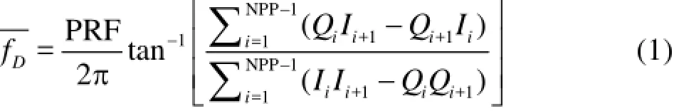
where NPP is the number of pulse pairs and the index i corresponds to a time step in theIandQsignal series, whose total number of elements is equal to the product of PRF and the total time of acquisition[30]. Therefore, the phase angle from which the Doppler frequency is determined has to be in the range-πto π, if it falls outside this range, phase wrapping or aliasing will occur[30].

Velocity data collected with the Vectrino Profiler and stored in orthogonal Cartesian coordinates were first transformed into their constituent beam velocities using the transformation matrix of the probe. The aliased phases were then recovered by multiplying these velocities by the quotient ofπand the ambiguity velocity, given by 4f0/cP RF, wherecis the speed of sound. For each beam, the resulting phase data were passed to the two-step non-continuous quality-guided path (TSNCQUAL) algorithm of Parkhurst et al.[26], which was designed for real-time usage during the Fourier profilometry of human patients undergoing radiotherapy treatment. In short, the algorithm is similar to the NCQUAL algorithm, except that a preprocessing step has been introduced to reduce the number of sorting and merging operations, yielding a significant performance increase[26]. After the beam velocities were dealiased, the transformation matrix was inverted to obtain the velocities in the original Cartesian coordinate system. Figure 3 shows an example of a severely aliased dataset, collected during unrelated flume experiments, before and after dealiasing.

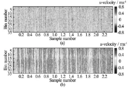
Fig.3 (a) Severely aliased Vectrino Profiler streamwise velocity (u)dataset from a laboratory flume experiment over a coarse, immobile, gravel bed. (b) The same dataset after dealiasing. Velocities were sampled for 240 s at 100 Hz, yielding 24 000 samples in each bin. For the 35 bins, the algorithm of Ref.[25] detected that between 11 631 and 14 020 of the samples were aliased.uof the aliased dataset ranged from 0.15 m/s to 0.213 m/s and RMSuranged from 0.157 m/s to 0.195 m/s.u of the dealiased dataset ranged from 0.283 m/s to 0.337 m/s and RMSuranged from 0.056 m/s to 0.083 m/s. Data were collected with a horizontal velocity range of 0.399 m/s. Dealiased statistics compared favorably to those collected with a horizontal velocity range of 0.901 m/s (no aliased samples,u ranged from 0.266 m/s to 0.328 m/s and RMSuranged from 0.054 m/s to 0.076 m/s). Unsurprisingly, the algorithm failed when the horizontal velocity range was set to a value ≈u

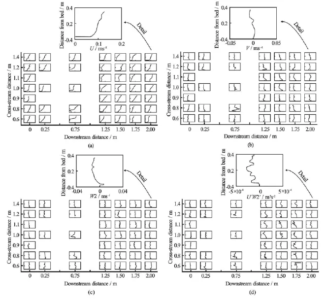
Fig.4 Stacked mean streamwise (U), cross-stream (V ), and vertical (W 2)velocity components and Reynolds stress (U ′W2′) profiles at 45 downstream and cross-stream locations, measured while the study area was fully vegetated. Flow was from right to left. The sketches show the approximate locations of the two L. digitata specimens, at coordinates of (0.46,0.67)and (0.81,1.16), respectively

1.2 Velocity filtering

The phase-space threshold filter of Wahl[27]is well-documented elsewhere and so will not be repeated here. Assuming a Gaussian spectrum for the acoustic backscatter, Zedel and Hay[28]defined an upper limit for the standard deviation of the phase as π/ norminv(1-ρ, where norminv(1-ρ) is the inverse normal function for a significance level of ρ, andGis the gain factor, which is 1.0 if the Vectrino Profiler is operated in single PRF mode orPRF2/(PRF1-PRF2)if the Vectrino Profiler is operated in dual PRF (extended velocity range) mode. As the correlation coefficient,R2, between successive samples obtained by the Vectrino Profiler is normalized, the minimum permissible correlation coefficient at a given significance level can then be estimated as[28]

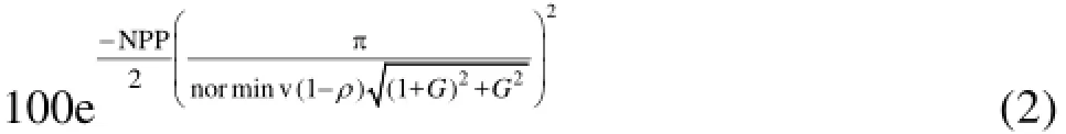
Velocities with R2values less than this were replaced with NaNs in the time series. Data suffering from aliasing also tended to suffer from low R2values and so this threshold was not applied to individual data points that had previously been dealiased. Note that Zedel and Hay[28]specified a constant value for norminv(1-ρ)and thatNPP=1. In the present work,ρ=0.001 and all data were collected using the single PRF mode; therefore G =1.0.

1.3 Time- and space-averaged statistics

The mean velocities, Reynolds stresses, turbulent kinetic energies and form-induced stresses presented in this paper were computed using only data that were retained after dealiasing and filtering (ignoring NaNs). On average 0.44% of data were dealiased and 7.89% of data were removed by filtering. Raw velocity data were time-averaged (denoted by a straight overbar), and then turbulent fluctuations (denoted by primes) were computed using the classical Reynolds decomposition:where uiis the instantaneous velocity in theithdirection. The head of the Vectrino Profiler comprises one transmitter and four receivers. It therefore provides two independent vertical velocity measurements:w1, which is estimated using data from receivers 1 and 3 (that are aligned in the streamwise direction), andw2, which is estimated using data from receivers 2 and 4 (that are aligned in the crossstream direction). Thus,i=1-4. Time-averaged data were then decomposed into spatially-averaged (denoted by angle brackets) and spatially fluctuating (denoted by a wavy overbar) components:Form-induced stresses were computed asuw.

2. Results and discussion

Upstream of the algae, the streamwise (u)velocity profile was approximately logarithmic with maxima of～0.10 m/s, while cross-stream(v)and vertical(w)flows were minimal (see Fig.4). Between the algae was a region of downwelling (w-velocity -0.035 m/s, Fig.4), while at the outer edges of the algae, counter-rotating velocity cells were generated (v|～0.04 m/s, Fig.4). Near-bed u-velocities were reduced to almost zero near and immediately downstream of the algae, but theu-velocities above the algae were unchanged (see Fig.4). The extent of the velocity reduction is controlled by the momentum-absorbing area of the algal blades[4]. The effect of the blades of the algae near mid-depth was therefore to cause the classical S-shaped velocity profile observed previously[2,5,17]for submerged vegetation. Immediately downstream of the algae, the flow above the blades behaves somewhat like a jet[19], decelerating in the downstream direction (Fig.4) and being redistributed by highly effective vertical momentum exchange[19]. This exchange was manifest in elevated magnitudes of u′ w′(～4× 10-4m2/s2) just above the elevation of the blades of the algae[4]near to and downstream of the algae (Fig.4), reflecting turbulence production[3,4,7]. However, near to the algae, the blades of the algae confined slow-moving near-bed fluid and thus limited momentum exchange with the overlying upper flow region (Fig.4)[4,23]. We infer that viscous diffusion caused Reynolds stress magnitudes to reduce with downstream distance as coherent vortices advected downstream and upwards (Fig.4). In typical mixing layers and flows over aquatic canopies, it has been observed that sweeps (Q4 events) dominate at the top of a canopy, whilst ejections (Q2) dominate above the canopy[7,21], and we expect that this is also true here. The spatial patterns ofu,v,w, andu′ w′imply that the flows around the algae at our field site are of intermediate relative submergence[23]. We may therefore identify four layers: (1) an upper flow region, in which the free surface restricts the development of a logarithmic layer and causes the flow to be dominated by the length scales and relatively coherent turbulence associated with layers 2 and 3[6], which together form the roughness sub-layer, (2) the form-induced (or dispersive) sub-layer, below the upper flow region and just above the canopy, where the time-averaged flow may be influenced by individual canopy elements and thus the terms u˜w˜may become nonzero, (3) the interfacial sub-layer, which occupies the region within the canopy where new contributors to the momentum balance appear: skin friction and form drag, and (4) a sub-canopy layer.

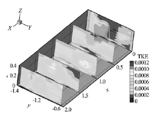
Fig.5 Spatial variation of turbulent kinetic energy (TKE) around twoL . digitata specimens. Contours at x=0.5 m and 1.0 m were interpolated from data atx=0.25 m and 0.75 m and 0.75 m and 1.25 m, respectively

Upstream from the algae, there were two regions of elevated turbulent kinetic energy (TKE) aligned with the algae[8], separated by a region of low TKE (Fig.5). Near to the algae and within the algae, these two regions of elevated TKE intensified and expanded (Fig.5), indicating increased turbulence, resulting from the shedding of vortices from the blades of the algae[6,7]. These patterns highlight the sensitivity of the spatial distribution of TKE to the position of measurements relative to algal stipes and blades[17]. Near to the bed, TKE-values remained low (Fig.5), suggesting the probable suppression of sediment transport.

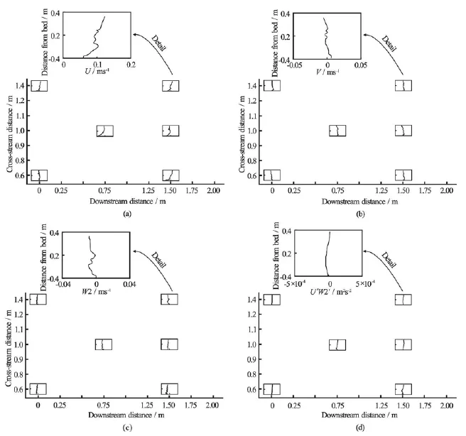
Fig.6 Stacked mean streamwise (U), cross-stream (V ), and vertical (W 2)velocity components and Reynolds stress (U ′W2′) profiles at five downstream and cross-stream locations, measured after removal of all macroalgae and large roughness elements (i.e., boulders)

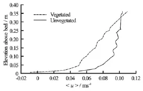
Fig.7 Double-averaged streamwise velocity profiles measured before (Vegetated) and after (Unvegetated) removal of all macroalgae and large roughness elements from the study area

After removal of the algae, cross-stream(v )and vertical(w)velocities were small within the footprint of the frame and values of u′ w′were uniformly <10-4m2/s2(Fig.6). This indicates the dominance of vegetation-induced over bedform- or bed roughnessgenerated shear[19]. Comparison of double-averaged streamwise velocities (u)indicates that in the vegetated case, the average velocity profile was significantly retarded below the elevation of the canopy (Fig.7), with the streamwise velocity exhibiting a near-linear increase for much of the water column (Fig.7). A linear double-averaged velocity profile is indicative of “k-type” roughness (isolated roughness flow), in which negative average velocity across a recirculation cell in the lee of roughness elements combines with a standard boundary layer profile along the remaining part of the gap between roughness elements[24]. This indicates that the algae are spaced sufficiently widely that there is no interaction betweentheir wakes[32]. However, there is no evidence of negative u-velocities in our dataset. Therefore, either a linear velocity profile is not necessarily dependent upon the formation of a recirculation cell or our sampling locations were too far downstream to capture the recirculation cell in the lee of the algae. In the unvegetated case, the velocity profile was more closely approximated by the law of the wall typical of a boundary layer (Fig.7). Note that the irregularities within these profiles are thought to reflect uncertainties in the calibration of the Vectrino Profiler and are not indicative of any underlying processes.

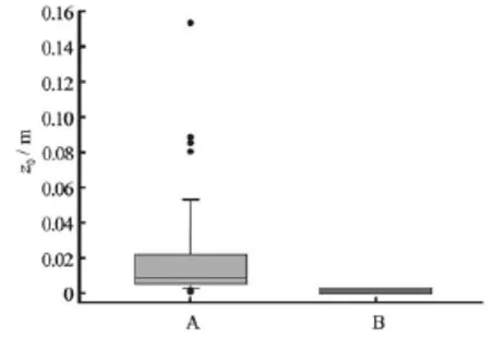
Fig.8 Box and whisker plot showing roughness heights,z0, computed by fitting the law of the wall to the stacked mean streamwise velocity profiles at all measurement locations when A) the study area was fully populated and B) after removal of all macroalgae and large roughness elements from the study area. The bounds of the boxes denote the 25th and 75th percentiles, error bars denote the 10th and 90th percentiles and solid dots denote outliers

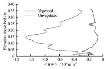
Fig.9 Vertical profiles of form-induced stresses (u˜w˜)estimated from velocity data measured before (Vegetated) and after removal of all macroalgae and large roughness elements (Unvegetated) from the study area

Fitting the law of the wall to individual u-velocity profiles (Figs.4 and 6), revealed a reduction in roughness height from～0.08 m-0.15 m near theL. digitata specimens to～0 m-0.006 m (Fig.8). This reduction was reflected in the reworking of the bed sediments by the current and the formation of ripples within the area. Note that the impact of macroalgae on roughness height was rather localized, with only those profiles in the immediate vicinity of algae exhibiting significantly increased roughness heights. Similarly, maximum form-induced stresses (-u˜w˜)occurred at an elevation of 0.146 m and were approximately an order of magnitude larger when macroalgae were present (1.07×10-4m2/s2) than when macroalgae and large roughness elements (i.e., boulders) had been removed from the study area (Fig.9). This pattern of negative form-induced stresses (hence upwards form-induced momentum transfer) is also consistent with “ktype” roughness (isolated roughness flow)[24].

3. Conclusions

In this paper, we used a profiling acoustic Doppler velocimeter to quantify the mean and turbulent flow fields around and between two Laminaria digitata thalli in a tidal inlet in Sør-Trøndelag, Norway. After plants were removed, velocity measurements were repeated over a sparser grid in order to differentiate between the impact of the macroalgae and bedforms on the local flow fields. The velocity and turbulence data presented herein are the first spatially-distributed measurements around, within and above a sparse, bladed macroalgae canopy and the first to employ the double-averaging methodology[23,24]. Custom phase unwrapping, or dealiasing, scripts, as well as spike and correlation filters were developed to process the data. This paper is the first to apply the state-of-the-art TSNCQUAL algorithm of Parkhurst et al.[26]to phase Doppler velocimetry data.

The data confirm that for “k-type” roughness (isolated roughness flow)[24], velocity and turbulence profiles are highly variable and dependent on the locations of roughness elements (in this case macroalgae) relative to the sampling location[17,19], emphasizing the need to employ the double-averaging methodology[23,24]. This sensitivity was also reflected in spatial patterns of turbulent kinetic energy. Macroalgae caused an increase in the roughness height from ～0 m-0.006 m to～0.08 m-0.15 m, closely matching the elevation of the maximum form-induced stresses. Thus, the roughness afforded by the macroalgae dominated bedform or bed roughness, caused reduced nearbed shear stresses and hence caused reduced transport of sandy sediments within the study area. Consequently, bedforms that are ubiquitous in sandy substrates were absent when the macroalgae were present but formed quickly once macroalgae were removed.

Future data analyses will attempt to couple the velocity measurements presented herein with in situ drag force and projected area measurements. The next phase of work involves repetition of the measurements within a 1:1 replica of the field prototype in the 11 m long×6 m wide Total Environment Simulator of the University of Hull. It is hoped that the datasets willallow a deeper understanding of the comparability of observations gained in the field and the laboratory, and the limitations and applicability of laboratory experiments.

Acknowledgements

The work described in this publication was supported by the European Community’s 7th Framework Programme through a grant to the budget of the Integrated Infrastructure Initiative HYDRALAB IV, Contract No. 261520. This document reflects only the authors’ views and not those of the European Community. This work may rely on data from sources external to the HYDRALAB project Consortium. Members of the Consortium do not accept liability for loss or damage suffered by any third party as a result of errors or inaccuracies in such data. The information in this document is provided “as is” and no guarantee or warranty is given that the information is fit for any particular purpose. The user thereof uses the information at its sole risk and neither the European Community nor any member of the HYDRALAB Consortium is liable for any use that may be made of the information. Field data collection would not have been possible without the assistance of the PISCES team of the HYDRALAB Consortium and field assistants: Tore Alstad, Olivier Eiff, Antti-Jussi Evertsen, Pierre-Yves Henry, Dan Parsons, Maike Paul, Jordan Royce, Adrian Teacă, and Costin Ungureanu. James Parkhurst of The Christie NHS Foundation Trust, Manchester, UK, kindly provided the C source code of his phase unwrapping algorithm, which allowed the lead author to port the algorithm to MATLAB.

[1] FOLKARD A. M. Vegetated flows in their environmental context: A review[J]. Proceedings of the Institution of Civil Engineering: Engineering and Computational Mechanics, 2010, 164(1): 3-24.

[2] NEPF H. M. Flow and transport in regions with aquatic vegetation[J]. Annual Review of Fluid Mechanics, 2012, 44(8): 123-142.

[3] NEPF H. M., VIVONI E. R. Flow structure in depthlimited, vegetated flow[J]. Journal of Geophysical Research, 2000, 105(C12): 28547-28557.

[4] WILSON C. A. M. E., STOESSER T. and BATES P. D. et al. Open channel flow through different forms of submerged flexible vegetation[J]. Journal of Hydraulic Engineering, ASCE, 2003, 129(11): 847-853.

[5] FOLKARD A. M. Hydrodynamics of model Posidonia oceanica patches in shallow water[J]. Limnology Oceanography, 2005, 50(5): 1592-1600.

[6] GHISALBERTI M., NEPF H. The structure of the shear layer in flows over rigid and flexible canopie [J]. Environment Fluid Mechanics, 2006, 6(3): 277-301.

[7] MALTESE A., COX E. and FOLKARD A. M. et al. Laboratory measurements of flow and turbulence in discontinuous distributions of ligulate seagrass[J]. Journal of Hydraulic Engineering, ASCE, 2007, 133(7): 750-760.

[8] SINISCALCHI F., NIKORA V. I. and ABERLE J. Plant patch hydrodynamics in streams: Mean flow, turbulence, and drag forces[J]. Water Resources Research, 2012, 48(1): 273-279.

[9] MILER O., ALBAYRAK I. and NIKORA V. et al. Biomechanical properties of aquatic plants and their effects on plant-flow interactions in streams and rivers[J]. Aquatic Sciences, 2012, 74(1): 31-44.

[10] JOHNSON A. S. Drag, drafting, and mechanical interactions in canopies of the red alga Chondrus crispus[J]. Biology Bulletin, 2001, 201(2): 126-135.

[11] LUHAR M., NEPF H. M. From the blade scale to the reach scale: A characterization of aquatic vegetative dra[J]. Advances Water Resources, 2013, 51(1): 305-316.

[12] SINISCALCHI F., NIKORA V. I. Flow-plant interactions in open-channel flows: A comparative analysis of five freshwater plant species[J]. Water Resources Research, 2012, 48(5): 2805-2814.

[13] LÓPEZ F., GARCÍA M. H. Mean flow and turbulence structure of open-channel flow through non-emergent vegetation[J]. Journal of Hydraulic Engineering, ASCE, 2001, 127(5): 392-402.

[14] GHISALBERTI M., NEPF H. M. The limited growth of vegetated shear layers[J]. Water Resources Research, 2004, 40(7): 196-212.

[15] NEPF H., GHISALBERTI M. Flow and transport in channels with submerged vegetation[J]. Acta Geophysica, 2008, 56(3): 753-777.

[16] SOULIOTIS D., PRINOS P. Effect of a vegetation patch on turbulent channel flow[J]. Journal of Hydraulic Research, 2011, 49(2): 157-167.

[17] NADEN P., RAMESHWARAN P. and MOUNTFORD O. et al. The influence of macrophyte growth, typical of eutrophic conditions, on river flow velocities and turbulence production[J]. Hydrological Processes, 2006, 20(18): 3915-3938.

[18] ZONG L., NEPF H. Flow and deposition in and around a finite patch of vegetation[J]. Geomorphology, 2010, 116(3-4): 363-372.

[19] SUKHODOLOV A. N., SUKHODOLOVA T. A. Case study: Effect of submerged aquatic plants on turbulence structure in a lowland river[J]. Journal of Hydraulic Engineering, ASCE, 2014, 136(7): 434-446.

[20] WHITE B., NEPF H. Shear instability and coherent structures in shallow adjacent to a porous layer[J]. Journal of Fluid Mechanics, 2007, 593: 1-32.

[21] CAMERON S. M., NIKORA V. I. and ALBAYRAK I. et al. Interactions between aquatic plants and turbulent flow: A field study using stereoscopic PIV[J]. Journal of Fluid Mechanics, 2013, 732: 345-372.

[22] KOEHL M. A. R., ALBERTE R. S. Flow, flapping, and photosynthesis of Nereocystis luetkeana: A functional comparison of undulate and flat blade morphologies[J]. Marine Biology, 1988, 99(3): 435-444.

[23] NIKORA V., MCLEAN S. and COLEMAN S. et al. Double-averaging concept for rough-bed open-channel and overland flows: Applications[J]. Journal of Hydraulic Engineering, ASCE, 2014, 133(8): 884-895.

[24] POKRAJAC D., MCEWAN I. and NIKORA V. Spatially averaged turbulent stress and its partitioning[J]. Experiments in Fluids, 2008, 45(1): 73-83.

[25] PAUL Maike, HENRY Pierre-Yves T. Evaluation of theuse of surrogate Laminaria digitata in eco-hydraulic laboratory experiments[J]. Journal of Hydrodynamics, 2014, 26(3): 374-383.

[26] PARKHURST J. M., PRICE G. J. and SHARROCK P. J. et al. Phase unwrapping algorithms for use in a true real-time optical body sensor system for use during radiotherapy[J]. Optices Applicata, 2011, 50(35): 6430-6439.

[27] WAHL T. L. Discussion of “Despiking acoustic Doppler velocimeter data” by Derek G. Goring and Vladimir I. Nikora[J]. Journal of Hydraulic Engineering, ASCE, 2003, 129(6): 484-487.

[28] ZEDEL L., HAY A. E. Resolving velocity ambiguity in multifrequency, pulse-to-pulse coherent Doppler sonar[J]. IEEE Journal of Oceanic Engineering, 2010, 35(4): 847-851.

[29] LHERMITTE R., SERAFIN R. Pulse-to-pulse coherent Doppler sonar signal processing techniques[J]. Journal of Atmospheric and Oceanic Technology, 1984, 1(4): 293-308.

[30] FRANCA M. J., LEMMIN U. Eliminating velocity aliasing in acoustic Doppler velocity profiler data[J]. Measurement Science Technology, 2006, 17(2): 313-322.

[31] LEMMIN U., ROLLAND T. Acoustic velocity profiler for laboratory and field studies[J]. Journal of Hydraulic Engineering, ASCE, 1997, 123(12): 1089-1098.

[32] FOLKARD A. M. Flow regimes in gaps within stands of flexible vegetation: Laboratory flume simulations[J]. Environment Fluid Mechanics, 2011, 11(3): 289-306.

* Biography: THOMAS Robert E. (1979-), Male, Ph. D., Post-Doctoral Research Associate