RAYLEIGH-TAYLOR INSTABILITY FORCOMPRESSIBLE ROTATING FLOWS∗

(段然)

School of Mathematics and Statistics,Central China Normal University,Wuhan 430079,China

E-mail:duanran@mail.ccnu.edu.cn

Fei JIANG(江飞)

College of Mathematics and Computer Science,Fuzhou University,Fuzhou 361000,China

E-mail:jiangfei0591@163.com

Junping YIN(尹俊平)

Institute of Applied Physics and Computational Mathematics,Beijing 100088,China

E-mail:yinjp@163.com

RAYLEIGH-TAYLOR INSTABILITY FOR
COMPRESSIBLE ROTATING FLOWS∗

Ran DUAN(段然)

School of Mathematics and Statistics,Central China Normal University,Wuhan 430079,China

E-mail:duanran@mail.ccnu.edu.cn

Fei JIANG(江飞)

College of Mathematics and Computer Science,Fuzhou University,Fuzhou 361000,China

E-mail:jiangfei0591@163.com

Junping YIN(尹俊平)

Institute of Applied Physics and Computational Mathematics,Beijing 100088,China

E-mail:yinjp@163.com

In this paper,we investigate the Rayleigh-Taylor instability problem for two compressible,immiscible,inviscid fows rotating with a constant angular velocity,and evolving with a free interface in the presence of a uniform gravitational feld.First we construct the Rayleigh-Taylor steady-state solutions with a denser fuid lying above the free interface with the second fuid,then we turn to an analysis of the equations obtained from linearization around such a steady state.In the presence of uniform rotation,there is no natural variational framework for constructing growing mode solutions to the linearized problem.Using the general method of studying a family of modifed variational problems introduced in[1], we construct normal mode solutions that grow exponentially in time with rate like where ξ is the spatial frequency of the normal mode and the constant c depends on some physical parameters of the two layer fuids.A Fourier synthesis of these normal mode solutions allows us to construct solutions that grow arbitrarily quickly in the Sobolev space Hk, and leads to an ill-posedness result for the linearized problem.Moreover,from the analysis we see that rotation diminishes the growth of instability.Using the pathological solutions, we then demonstrate the ill-posedness for the original non-linear problem in some sense.

Rayleigh-Taylor instability;rotation;Hadamard sense

2010 MR Subject Classifcation35L65;35L60

1 Introduction

Hydrodynamic instabilities at the interface of two materials of diferent densities are a critical issue in high energy density physics(HEDP).The Rayleigh-Taylor instability(RTI)occurswhen a fuid accelerates another fuid of high density[2-4].The RTI is ubiquitous in HEDP, such as high Mach number shocks and jets,radiative blast waves and radioactively driven molecular clouds,gamma-ray bursts and accreting black holes,etc.Due to the importance in physics mentioned above,there have been many studies related to RTI from both physical and numerical simulation points of view in the literature.As for the analytical investigation concerning the linearized problems,we refer to the monographs[5,6]in which the authors studied the efects on RTI of various physical and geometric quantities including surface tension,viscosity as well as the shape of the domain and so on.But unfortunately,few analytical results concerning the nonlinear problems showed up until the year of 1987 in which Erban[7]proved the ill-posedness of the equations of motion for a perfect fuid with free boundary.Then he adapted this approach to obtain the nonlinear ill-posedness of both RTI and Helmholtz instability problems for two-dimensional incompressible,immiscible,inviscid fuids without surface tension[8].In 2011,Y.Guo and I.Tice[9]established a variational framework for nonlinear instabilities. They constructed solutions that grow arbitrarily quickly in the Sobleve space by the method of Fourier synthesis,which leads to an ill-posedness to the perturbed problem.later on,for this stratifed fuids,several works studied the efects of viscosity and surface tension on the RTI for incompressible and compressible fuids(see[1,10-13]).As for the RTI for the equations of magnetohydrodynamics,please refer to[14-17]and[18-21]for relevant background of MHD, where the authors studied the efect of the magnetic feld.Besides the stratifed fuids,we also refer to[22-26]for the continuous fuids.

While,if the two fuids are all subject to a uniform rotation with an constant angular velocity,how does this rotation infuent the RTI?Stabilize it or make it more unstable?To the best of our knowledge,physicists[5,6]showed that rotation can only slow down the growth rate of the disturbance a little bit,but not prevent the incompressible fuids from becoming unstable.Now,an interesting question is whether it is still true for compressible fows?

In this paper,for inviscid compressible fows without the centrifugal force,we frst prove that the linearized system is unstable in the Hadamard sense.Then,we establish the ill-posedness for the original non-linear problem in some sense.

Next,we formulate the problem in details for further discussion.

1.1 Formulation in Eulerian Coordinates

We suppose that the fuids are confned between two rigid planes.As in[9],we denote this infnite slab by Ω=R2×(-m,l)⊂R3.The fuids are separated by a moving free interface Σ(t)(t≥0)that extends to infnity in every horizontal direction.The interface divides Ω into two time-dependent,disjoint,open subsets Ω±(t),so that Ω=Ω+(t)∪Ω-(t)∪Σ(t)and Σ(t)=¯Ω+(t)∩¯Ω-(t).The motion of the fuids is driven by the constant gravitational feld along e3-the x3direction,g=(0,0,-g)with g＞0 and the rotation with an angular velocity ω=(0,0,ω)about the vertical direction.Quantities describing fuids are their density and velocity,which are given for each t≥0 by,respectively,

We shall assume that at a given time t≥0 these functions have well-defned traces onto Σ(t).

The fuids are governed by the following equations:

for t＞0 and x∈Ω±(t).Here we have written g＞0 for the gravitational constant,e3=(0,0,1) for the vertical unit vector,and-ge3for the acceleration due to gravity,2ρ±(ω×u±)represents the Coriolis force,while the centrifugal force ρ±∇|ω×x|2/2,like in[27,28],is neglected on the basis of a standard argument which indicates that the motion is dominated by gravitation and the centrifugal force is small.

In particular,this requires that the pressure laws be distinct,i.e.,p-/=p+.

Now,we prescribe the jump conditions that,from the physical point of view,both normal component of the velocity and the pressure are continuous across the free interface(since no surface tension is taken into account),see[5,29].Therefore,the jump conditions at the free interface read as

for each t＞0,where we have denoted the normal vector to Σ(t)by ν,the trace of a quantity f on Σ(t)by f|Σ(t)and the interfacial jump by

On the fxed boundaries,we consider that the normal component of the fuid velocity vanishes,that is,

The motion of the free interface is coupled to the evolution equations for the fuids(1.1) by requiring that the interface be advected with the fuids.This means that the velocity of the interfcae is given by(u·ν)ν.Since the normal component of the velocity is continuous across the surface there is no ambiguity in writing u·ν.The tangential components of u±need not be continuous across Σ(t),and indeed there may be jumps in them.This allows possible slipping: the upper and lower fuids moving in diferent directions tangent to Σ(t).Since only the normal component of the velocity vanishes at the fxed upper and lower boundaries,{x3=l}and {x3=-m},the fuids may also slip along the fxed boundaries.

To complete the statement of the problem,we must specify initial conditions.We give the initial interface Σ(0)=Σ0,which yields the open sets Ω±(0)on which we specify the initial data for the density and the velocity

To simply the equations we introduce the indicator function χ and denote

Hence the equations(1.1)are replaced by

for t＞0 and x∈Ω/Σ(t).It will be convenient in our subsequent analysis to rewrite the momentum equations in(1.2)by using the enthalpy function

The properties of p ensure that h∈C∞(0,∞).Thus,(1.2)can be rewritten as

In the subsequent analysis it will be convenient to use the notation

1.2 Steady-state Solution

In order to produce RTI,we frst seek a steady-state solution with u±=0 and the interface given by{x3=0}for all t≥0.Then Ω+≡Ω+(t):=R2×(0,l),Ω-≡Ω-(t)=:R2×(-m,0) for all t≥0,and the equations reduce to the ODE

subject to the jump condition

Such a solution depends only on x3,so we consolidate notation by assuming that ρ±are the restrictions to(0,l)and(-m,0)of a single function ρ0=ρ0(x3)that is smooth on(-m,0)and (0,l)with a jump discontinuity across{x3=0}.

From the assumption of the pressure function p and the defnition of the set Z,there exist two positive constants l and m and a solution ρ0to(1.4)-(1.5)such that

·ρ0is bounded above and below by positive constants on(-m,l),and ρ0is smooth when restricted to(-m,0)or(0,l).

Please refer to[9,Section 1.2]for more details concerning construction of such a solution. In this paper,we always assume that l,m and the solution ρ0satisfy the above properties.

1.3 Formulation in Lagrangian Coordinates

We think of the Eulerian coordinates as(t,y)with y=η(t,x),whereas we think of Lagrangian coordinates as the fxed(t,x)∈R+×Ω,this implies that Ω±(t)=η±(t,Ω±)and that Σ(t)=η+(t,{x3=0}),i.e.,that the Eulerian domains of upper and lower fuids are the image of Ω±under the mapping η±and that the free interface is parameterized by η+(t,·)restricted to R2×{0}.In order to switch back and forth from Lagrangian to Eulerian coordinates we assume that η±(t,·)is invertible.Since the upper and lower fuids may slip across one another, we must introduce the slip map S±:R+×R2→R2×{0}⊂R2×(-m,l)defned by

Setting η=χ+η++χ-η-,we defne the Lagrangian unknowns

Since the boundary jump conditions in Eulerian coordinates are phrased in terms of jumps across the interface,the slip map must be employed in Lagrangian coordinates.The jump conditions in Lagrangian coordinates are

where we have written n=ν◦η,i.e.,

for the normal to the surface Σ(t)=η+(t,{x3=0}).Note that we could just as well have phrased the jump conditions in terms of the slip map S+and defned the interface and its normal vector in terms of η-.Finally,we require

Note that since∂tη=v,which implies that η+(t,x′,l)∈{x3=l}for all t≥0,i.e.,that the part of the upper fuid in contact with the fxed boundary{x3=l}never fows down from the boundary.It may, however,slip along the fxed boundary,since we do not require v+(t,x′,l)·ei=0 for i=1,2. A similar result holds for η-at the lower fxed boundary{x3=-m}.

In the steady-state case,the fow map is the identity mapping,η=Id,so that v=u and q=ρ.This means that the steady-state solution,ρ0,constructed above in Eulerian coordinates is also a steady state in Lagrangian coordinates.Now we want to linearize the equations around the steady-state solution v=0,η=Id,q=ρ0,for which S-=Id{x3=0}and A=I.The resulting linearized equations read as

The corresponding linearized jump conditions are

while the boundary conditions are

1.4 Main Results

Before stating the frst result concerning linear problem,we defne some terms that will be used throughout the paper.For a function f∈L2(Ω),we defne the horizontal Fourier transform via

By the Fubini and Parseval theorems,we have that

For a function f defned on Ω we write f+for the restriction to Ω+=R2×(0,l)and f-for the restriction to Ω-=R2×(-m,0).For s∈R,defne the piecewise Sobolev space of order s by

for I-=(-m,0)and I+=(0,l).The main diference between the piecewise Sobolev space Hs(Ω)and the ususal Sobolev space is that we do not require functions in the piecewise Sobolev space to have weak derivatives across the set{x3=0}.Now,we may state our result on the linear problem as follows:

Theorem 1.1 shows discontinuous dependence on the initial data.More precisely,there is a sequence of solutions with initial data tending to 0 in Hk(Ω),but which grow to be arbitrarily large in Hk(Ω).Here we describe the framework of the proof,which is inspired by[9].First the resulting linearized equations have coefcient functions that depend only on the vertical variable,x3∈(-m,l).This allows us to seek“normal mode”solutions by taking the horizontal Fourier transform of the equations and assuming that the solution grows exponentially in time by the factor eλ(|ξ|)t,where ξ∈R2is the horizontal spatial frequency and λ(|ξ|)＞0.We show in Theorem 2.9 that λ(|ξ|)→∞in some unbounded domain,the normal modes with a higher spatial frequency grow faster in time,thus providing a mechanism for RTI.Indeed, we can form a Fourier synthesis of the normal mode solutions constructed for each spatial frequency ξ to construct solutions of the linearized equations that grow arbitrarily quickly in time,when measured in Hk(Ω)for any k≥0.Compared with[9],the main difculty here of constructing this growing solutions lies in building the variational structure of the linearized equations,because the natural variational structure breaks down in the presence of the rotation term.This difculty will be circumvented in Section 2 by employing an approach that was used frst by Guo and Tice[4]to overcome a similar difculty arising from viscous compressible fuids, and later adapted by Jiang,Jiang and Wang[7]in a nontrivial way to construct growing mode solutions for viscous incompressible fuids with magnetic feld.Due to presence of the rotating term,we have to impose stronger restrictions on the parameter s and the spatial frequency ξ in order to obtain the existence result(2.21)and the lower boundedness of λ2in(2.24)for the rotating case.In addition,the auxiliary function Φ(s)(see[1,(3.52)]),constructed by Guo and Tice to show(2.21),can not be applied to our case,and we have to construct a new auxiliary function F(s)in order to get(2.21).At last,in Section 3 we show a connection between the growth rate of solutions to the linearized equations and the eigenvalues λ(ξ),which then gives rise to a uniqueness result(see Theorem 3.4).In spite of the uniqueness,the linear problem is still ill-posed in the sense of Hadamard in Hk(Ω)for any k,since solutions do not depend continuously on the initial data.

With the linear ill-posedness established,we can obtain the ill-posedness of the fully nonlinear problem in some sense.We rephrase the nonlinear equations(1.7)in a perturbation formulation around the steady state,that is,v=0,η=η-1=Id,q=ρ0with A=I and S-=S+=Id{x3=0}.Let

In order to deal with the term h(q)=h(ρ0+σ)we introduce the Taylor expansion

where the remainder term is defned by

Then(1.7)can be written for~η,v,σ as

where Ididenotes the i-th component of Id,i=1,2.We require the compatibility between ζ and~η given by

The jump conditions across the interface are

where the slip map(1.6)is rewritten as

Finally,we require the boundary condition

We collectively refer to(1.12)-(1.16)as the perturbed problem.To shorten notation,for k≥0 we defne

In order to prove the ill-posedness for the perturbed problem by contradiction,we state a defnition introduced in[9]:

Defnition 1.2We say that the perturbed problem has property EE(k)for some k≥3 if there exist δ,t0,C＞0 and a function F:[0,δ)→R+satisfying

(4)we have the estimate

Here the EE stands for existence and estimates,i.e.,local-in-time existence of solutions for small initial data,coupled to L∞(0,t0;H3(Ω))estimates in terms of Hk(Ω)-norm of the initial data.If we were to add the additional condition that such solutions be unique,then this trio could be considered a well-posedness theory for the perturbed problem.

We can now show that property EE(k)cannot hold for any k≥3.The proof utilizes the Lipschitz structure of F to show that property EE(k)would give rise to certain estimates of solutions to the linearized equations(1.8)that cannot hold in general because of Theorem1.1.

Theorem 1.3The perturbed problem does not have property EE(k)for any k≥3.

Remark 1.4Theorems 1.1 and 1.3 show that rotating angular velocity ω can not prevent the linear and nonlinear RTI in the sense described in Theorems 1.1 and 1.3,respectively. However,in the construction of the normal mode solution to the linearized system in Subsection 2.2,the rotation dose have a stabilizing efect on the growth rate λ for sufciently large fxed |ξ|.In fact,in Subsection 2.2,we know that there exists a couple

such that

Obviously,φ0≡/0.On the other hand,we denote the growth rate by λ0for the equations of compressible inviscid fuids without rotation(i.e.,ω=0),that is

Thus we have

which implies λ＜λ0.

2 Construction of a Growing Solution to(1.8)

We wish to construct a solution to the linearized equations(1.8)that has a growing Hknorm for any k.We will construct such solutions via Fourier synthesis by frst constructing a growing mode for a fxed spacial frequency.

2.1 Growing Mode and Fourier Transform

with the corresponding jump conditions

and the boundary conditions

Since the jump only occurs in the e3direction,we are free to take the horizontal Fourier transform,which we denote with eitherˆ·or F,to reduce to a system of ODEs in x3for each fxed spacial frequency.

We take the horizontal Fourier transform of w1,w2,w3in(2.1)and fx a spacial frequency ξ=(ξ1,ξ2)∈R2.Defne the new unknowns

To write down the equations for φ,θ,ψ,we denote′=d/dx3to arrive at the following system of ODEs

along with the jump conditions

and boundary conditions

Putting this identity into(2.2),we arrive at

along with the jump conditionsand boundary conditions(2.3).

In the absence of rotation(ω=0)and for a fxed spatial frequency ξ/=0,the equations (2.4),(2.5)and(2.3)can be viewed as an eigenvalue problem with eigenvalue-λ2.Such a problem has a natural variational structure that allows us to construct solutions via the direct method and a variational characterization of the eigenvalues via

This variational structure was essential to the analysis in[9],where the ill-posedness results for both the inviscid linearized problem and the inviscid non-linear problem((1.12)with ω=0) were shown.Unfortunately,when rotation is present,the natural variational structure breaks down.In order to circumvent this problem and restore the ability to use the variational method, frst we artifcially remove the dependence of(2.4)on λ-2by defning s:=λ-2＞0,and then consider a family(s＞0)of the modifed problems given by

along with the jump conditions

and boundary conditions(2.3).

2.2 Construction of a Solution to(2.6)

In the following,we establish the variation framework by formulating constrained minimization.Multiplying(2.6)1and(2.6)2by φ and ψ,respectively,we add the resulting equations, integrate over(-m,l),integrate by parts,and apply the boundary and jump conditions to deduce that

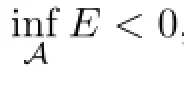
We want to show that the infmum of E(φ,ψ)over the set A can be achieved and is negative, and that the minimizer solves the problem(2.6),(2.7)and(2.3).Notice that by employing the identity-2ab=(a-b)2-(a2+b2)and the constraint on J(φ,ψ),we may rewrite

In order to emphasize the dependence on s∈(0,∞),we will sometimes write

By inequality(2.8)we have

In particular,we have

ProofSince both E and J are homogeneous of degree 2,it sufces to show that

We assume that φ=-ψ′/|ξ|,such that the frst integrand term in E(φ,ψ)vanishes,that is,

where we have used the fact that ρ0solves(1.4).Notice that[|ρ0|]＞0 so that the right-hand side is not positive defnite.From(2.12)we see that the rotation term diminishes obviously the growth of instability.

Thus,we can estimate that

for some positive constants C1,A4and A5depending on the same parameters,but not on|ξ|.

Obviously,there exist a sufciently large positive constant R1＞0 and a positive constant C0depending on A4and A5,such that

Inserting(2.17)into(2.16),we obtain

which implies the desired conclusion.

The key point in the proof argument of Proposition 2.1 is to construct a pair(φ,ψ),such that

which in particular requires that ψ(0)/=0.We can show that this property is satisfed by any (φ,ψ)∈A with E(φ,ψ)＜0.

Lemma 2.2Suppose that(φ,ψ)∈A satisfes E(φ,ψ)＜0.Then ψ(0)/=0.

ProofA completion of square allows us to write

Thus,similarly to(2.12),we can rewrite the energy as

from which we deduce that if E(φ,ψ)＜0,then ψ(0)/=0.?

From now on,we denotewhere the constants R1,C0and C1are from Proposition 2.1.Next,we can show that a minimizer exists and that the minimizer satisfes(2.6),(2.7)and(2.3)for each(ξ,s)∈M in the same manner as in[1].

Proposition 2.3For any fxed(ξ,s)∈M,E achieves its infnimum on A.

All that remains is to show(φ,ψ)∈A.

which is a contradiction since(αφ,αψ)∈A.Hence J(φ,ψ)=1 so that(φ,ψ)∈A.?

Proposition 2.4Let(ξ,s)∈M,and(φ,ψ)∈A be the minimizer of E constructed in Proposition 2.3.Letµ:=-λ2:=E(φ,ψ).Then φ,ψ satisfy

along with the jump conditions(2.5)and boundary conditions(2.3).Moreover,the solutions are smooth when restricted to either(-m,0)or(0,l).

and note that j(0,0)=1.Moreover,j is smooth,and

Thus,by the inverse function theorem,we can fnd a C1-function r=σ(t)in a neighborhood of 0,such that σ(0)=0 and j(t,σ(t))=1.We may diferentiate the last equation to infer that

Since(φ,ψ)is a minimizer of E over A,one has

which implies that

The above equation,by rearranging and plugging in the value of σ′(0),can be rewrite as

where the lagrange multiplier(eigenvalue)isµ=E(φ,ψ).

The next result establishes continuity property of the eigenvalueµ(s)which will be used in fnding a s with s=1/λ2(s)in Theorem 2.7.

ProofFix a compact interval I=[a,b]⊂(0,∞),and fx any pair(φ0,ψ0)∈A.We may decompose E according to

The non-negativity of E1implies that E is non-decreasing in s with fxed(φ,ψ)∈A.

Now,by Proposition 2.3,for each s∈(0,∞)we can fnd a pair(φs,ψs)∈A so that

We deduce from the non-negativity of E1,the minimality of(φs,ψs)and the equality(2.8)thatfor all s∈Q,which implies that there exists a constant 0＜K=K(a,b,φ0,ψ0,g,|ξ|)＜∞, such that

Let si∈Q for i=1,2.Using the minimality of(φs1,ψs1)compared to(φs2,ψs2),we see that

Recalling the decomposition(2.19),we can bound

Putting these two inequalities together and employing(2.20),we conclude that

Reversing the role of the indices 1 and 2 in the derivation of the above inequality gives the same bound with the indices switched.Therefore,we deduce that

which completes the proof of Proposition 2.5.

To emphasize the dependence on the parameters,we write

In view of Propositions 2.4 and 2.1,we can state the following existence result of solutions to (2.6),(2.7)and(2.3)for each(ξ,s)∈M.

Proposition 2.6For each(ξ,s)∈M,there exists a solution φs(|ξ|,x3),ψs(|ξ|,x3)with λ=λ(|ξ|,s)＞0 to the problem(2.6)along with the corresponding jump and boundary conditions.Moreover,these solutions ψs(|ξ|,0)/=0 and the solutions are smooth when restricted to either(-m,0)or(0,l).

In order to prove λ→+∞as|ξ|→+∞,and give the existence of solutions to the original problem(2.5),(2.4)and(2.3),we shall further restrict ξ to satisfy

where C0,C1and R1are the constants from Proposition 2.1.Thus we have the following conclusion.

Theorem 2.7For each ξ with|ξ|＞R2≥R1,there exists an s∈(0,s1):=(0,C0R2/C2), such that

Remark 2.8It is easy to check that(ξ,s)∈M for any|ξ|＞R2and s∈(0,s1).

ProofRecalling-λ2(s)=µ(s),we defne

According to Proposition 2.5,F(s)is continuous.Moreover,we have

Now if there exists a¯s∈(0,s1)such that

then combining(2.22)with(2.23),we can fnd s∈(0,¯s)such that F(s)=0,i.e.,(2.21)holds. In the following,we verify(2.23).

According to(2.11)and the fact C2＞C1,we see that

which yields

2.3 Construction of a Solution to(2.2)

We may now use Theorem 2.7 to think of s=s(|ξ|),since we can fnd s∈S so that(2.21) holds.As such we may also write λ=λ(|ξ|)from now on.

Once Theorem 2.7 is established,we can combine it with Proposition 2.6 to obtain immediately a solution to(2.4),and in turn a solution to(2.2)for each spacial frequency ξ with |ξ|＞R2.

Theorem 2.9For ξ∈R2with|ξ|＞R2,there exists a solution φ=φ(ξ,x3),θ=θ(ξ,x3), ψ=ψ(ξ,x3)and λ=λ(|ξ|)＞0 to(2.2),such that ψ(0)/=0.The solution is smooth when restricted to(-m,0)or(0,l),and it is equivariant in ξ in the sense that if R∈SO(2)is a rotation operator,then

where C0,C1and R2are the constants from Proposition 2.1 and Theorem 2.7.

ProofIn view of Theorem 2.7 and Proposition2.6,there exists a solution(φ(|ξ|),ψ(|ξ|),θ≡0)to(2.2)for the fxed frequency given by(|ξ|,0)with|ξ|＞R2.Thus we may fnd a rotation operator R∈SO(2)so that R(ξ)=(|ξ|,0).Defne(φ(ξ,x3),θ(ξ,x3))=R-1(φ(|ξ|,x3),0)and ψ(ξ,x3)=ψ(|ξ|,x3).This gives a solution to(2.2)for any frequency ξ with|ξ|＞R2.The equivalence in ξ follows from the defnition.

We proceed to estimate(2.11).According to(2.14),for|ξ|＞R2≥R1,one has

The fact that s=1/λ2from Theorem 2.7 combined with(2.25)results in

which leads to

On the other hand,in view of Theorem 2.7,we fnd that

which implies that(2.27)does not hold.Hence,λ2has to satisfy(2.26).

For|ξ|＞(C1+1)/C0,we have

By virtue of(2.26)and(2.28),the estimate(2.24)is obtained by denoting C3=C1/2.?

Next,we derive an estimate for the Hk-norm of the solutions(φ,ψ)with|ξ|varying,which will be used in the proof of Theorem 2.11 when integrating solutions in a Fourier synthesis.

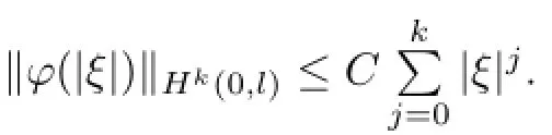
Lemma 2.10Let φ(|ξ|),ψ(|ξ|)be the solutions to(2.6)constructed in Theorem 2.9.Let R2,C0,C1,C3＞0 be the constants from Theorem 2.9.Fix R0=max{(C1+1)/C0,2/C3,R2,1}∈(0,∞).Then for any ξ with|ξ|≥R0and for each k≥0,there exists a constant Ak＞0 depending on ρ0,p,g,ω,l and m,such that

Also,there exists a constant B0＞0 depending on the same parameters,such that for any |ξ|＞0,

ProofWe begin with the proof of(2.29).For simplicity we will derive an estimate of the Hk-norm on the interval(0,l)only.A bound on(-m,0)follows similarly,and the desired result follows from adding the two estimates together.First note that the choice of R0,when combined with Theorem 2.9 and(2.10),implies that

Also keep in mind that ρ0is smooth on each interval(0,l)and(-m,0)and bounded from above and below.Throughout the proof we denote by C a generic positive constant depending on the appropriate parameters.We proceed by induction on k.For k=0 the fact that (φ(|ξ|),ψ(|ξ|))∈A implies that there is a constant A0＞0 depending on the various parameters, so that

Suppose now that the bound holds for some k-1≥0,i.e.,

These equations,together with(2.31)and the fact that|ξ|＞1,yield that

On the other hand,the defnition of w(|ξ|)implies that

from which we get

for some constant Ak＞0 depending on the parameters,i.e.,the bound holds for k.By induction,the bound holds for all k≥0.Finally,(2.30)follows from the fact that(φ(|ξ|),ψ(|ξ|))∈A and ρ0is bounded from above and below.?

2.4 Fourier Synthesis

Inspired by[9],we will use the Fourier synthesis to build growing solutions to(1.8)out of the solutions constructed in the previous section for fxed spacial frequency ξ∈R2.The solutions will be constructed to grow in the piecewise sobolev space of order k,Hk,defned by (1.9).

where φ,θ,ψ and π are solutions to(2.2).Writing x′·ξ=x1ξ1+x2ξ2,we defne

where we have defned λ(|ξ|)=φ(ξ,x3)≡θ(ξ,x3)≡ψ(ξ,x3)≡0 if|ξ|≤R0.Then η,v,q are real-valued solutions to the linearized equations(1.8)along with the corresponding jump and boundary conditions.For every k∈N,we have the estimate

ProofFor each fxed ξ∈R2,

gives a solution to(1.8).Since supp(f)⊂B(0,R4)/B(0,R3),Lemma2.10 results in

These bounds imply that the Fourier synthesis of the solutions given by(2.33)is also a solution to(1.8).The bound(2.34)follows from Lemma 2.10 with arbitrary k≥0 and the fact that f is compactly supported.From(2.31),the estimates(2.35)follow.?

3 Ill-posedness for the Linear Problem

We assume that η,v,q are the real-valued solutions to(1.8)along with the corresponding jump and boundary conditions established in Theorem 1.1.Furthermore,suppose that the solutions are band-limited at radius R＞0,i.e.,that

Diferentiating the second equation in(1.8)with respect to times t and eliminating the η term by using the frst equation,we obtain

along with the jump and boundary conditions

By the standard energy estimate procedure(see[1,Section 3]),we can establish three energy estimates in the following which ensure the uniqueness result in Theorem 3.4.

Lemma 3.1For solutions to(3.1)it holds that

Lemma 3.2Let v∈H1(Ω)be band-limited at radius R＞0 and satisfy the boundary conditions v3(t,x′,-m)=v3(t,x′,l)=0.Then

where the value of Λ(R),depending R,is given by(4.2)in[9,Section 4.1].

Proposition 3.3Let v be a solution to(3.1)along with the corresponding jump and boundary conditions that is also band-limited at radius R＞0.Then

for a constant C=C(ρ0,l,m,p,g,Λ(R))＞0,where the value of Λ(R),depending R,is given by(4.2)in[9,Section 4.1].

Similar to[9],once we get Proposition 3.3,through constructing the horizontal spatial frequency projection operator,we can obtain the uniqueness result.Here we give the proof for the reader’s convenience.

where F·=ˆ·denotes the horizontal Fourier transform in x′.It is easy to see that PRsatisfes the following.

(1)PRf is band-limited at radius R.

(2)PRis a bounded linear operator on Hk(Ω)for all k≥0.

(3)PRcommutes with partial diferentiation and multiplication by functions depending only on x3.

(4)PRf=0 for all R＞0 if and only if f=0.

Now we are able to prove the uniqueness results on η,v and q.

Theorem 3.4Assume that(η1,v1,q1)and(η2,v2,q2)are two solutions to(1.8).Then η1=η2,v1=v2and q1=q2.

ProofIt sufces to show that solutions to(1.8)with 0 initial data remain 0 for t＞0. Suppose that η,v are solutions with vanishing initial data.Fix R＞0 and defne ηR=PRη, vR=PRv,qR=PRq.The properties of PRshow that ηR,vR,qRare also solutions to(1.8)but that they are band-limited at radius R.Turning to the second order formulation,we fnd that vRis a solution to(3.1)with initial data vR(0)=∂tvR(0)=0.We may then apply Proposition 3.3 to deduce that

which shows that ηR(t),vR(t)and qR(t)all vanish for t≥0.Since R is arbitrary,it must hold that η(t),v(t)and q(t)also vanish for t≥0.?

The solutions to the linear problem(1.8)constructed in Theorem 2.11 are sufciently pathological to give rise to a result showing that the solutions depend discontinuously on the initial data.Then,in spite of the previous uniqueness result,we obtain that the linear problem is ill-posed in the sense of Hadamard.Next,we prove Theorem 1.1.

Similar to[9],once we get the pathological solutions to the linear problem(1.8)constructed in Theorem2.11,we are able to show that the solutions depend discontinuously on the initial data described in Theorem 1.1.Here we give the proof for the reader’s convenience.

We may now apply Theorem 2.11 with fn,R3=R(n),and R4=R(n)+1 to fnd ηn,vn,qnthat solve(1.8)with the corresponding jump and boundary conditions,such that ηn,vn,qn∈Hj(Ω)for all t≥0.By(2.34)and the choice of fnsatisfying(3.2),we fnd that(1.10)holds for all n.

On the other hand,we have

from which(1.11)follows.

4 Proof of Theorem 1.3

The proof is similar to[9]under necessary modifcations.We argue by contradiction. Suppose that the perturbed problem has property EE(k)for some k≥3.Let δ,t0and C＞0 be the constants and function provided by the property EE(k).Fix n∈N so that n＞C, applying Theorem 1.1 with this n,T0=t0/2,k≥3 and α=1,we can fnd¯η,¯v,¯σ solving (1.8),such that

with boundary conditions

and

According to the bound(4.3)and the sequential weak-∗compactness,we have that up to the extraction of a subsequence(which we still denote using only∈),

By lower semicontinuity we know that

and∈＜1/(2K1),where K1＞0 is the best constant in the inequality‖FB‖H4≤K1‖F||H4‖B‖H4 for 3×3 matrix-valued functions F,B.The former condition implies that ρ0+∈¯σ∈is bounded from above and below by positive quantities,whereas the latter guarantees that¯B∈is welldefned and uniformly bounded in L∞(0,t0;H2(Ω))since

A straightforward calculation,recalling(4.5)and(4.6),shows that

We now turn to some convergence results for the jump conditions.We begin with the second equation in(1.14),which we expand using the mean-value theorem to get

For the second equation in(1.14)we frst write the normal at the interface as n∈=N∈/|N∈| with

As∈→0 we have|N∈|＞0,so we may rewrite the frst equation in(1.14)as

from which we fnd that

This strong convergence,together with the convergence results(4.8)and(4.10)and the equation∂t¯η∈=¯v∈,implies that

and that

as well.

Hence we may chain together inequalities(4.1)and(4.5)to get

which is a contradiction.Therefore,the perturbed problem does not have property EE(k)for any k≥3.?

[1]Guo Y,Tice I.Linear Rayleigh-Taylor instability for visccous,compressible fuids.SIAM J Math Anal, 2011,42:1688-1720

[2]Rayleigh L.Analytic solutions of the Rayleigh equations for linear density profles.Proc London Math Soc, 1883,14:170-177

[3]Rayleigh L.Investigation of the character of the equilibrium of an incompressibleheavy fuid of variable density.Scientifc Papaer,1900,II:200-207

[4]Taylor G I.The stability of liquid surace when accelerated in a direction perpendicular to their planes. Proc Roy Soc A,1950,201:192-196

[5]Chandrasekhar S.Hydrodynamic and Hydromagnetic Stability.The International Series of Monographs on Physics.Oxford:Clarendon Press,1961

[6]Wang J.Two-Dimensional Nonsteady Flows and Shock Waves(in Chinese).Beijing:Scientifc Press,1994

[7]Erban D.The equations of motion of a perfect fuid with free boundary are not well posed.Comm Partial Diferential Equations,1987,12:1175-1201

[8]Erban D.Ill-posedness of the Rayleigh-Taylor and Helmholtz problems for incompressible fuids.Comm Partial Diferential Equations,1988,13:1265-1295

[9]Guo Y,Tice I.Compressible,inviscid Rayleigh-Taylor instability.Indiana Univ Math J,2011,60:677-712

[10]Pruess J,Simonett G.On the Rayleigh-Taylor instability for the two-phase Navier Stokes equations.Indiana Univ Math J,2010,59(3):1853-1871

[11]Wang Y J,Tice I.The viscous surface-internal wave problem:nonlinear Rayleigh-Tayor instability.Comm Partial Diferential Equations,2012,37:1967-2028

[12]Jiang F,Jiang S,Wang W W.On the Rayleigh-Taylor instability for two uniform viscous incompressible fows.Chinese Ann Math B,2014,35(6):907-940

[13]Jiang F,Jiang S,Wang Y J.On the Rayleigh Taylor instability for the incompressible viscous magnetohydrodynamic equations.Comm Partial Diferential Equations,2014,39:399-438

[14]Duan R,Jiang F,Jiang S.On the Rayleigh-Taylor instability for incompressible,inviscid magnetohydrodynamic fows.SIAM J Appl Math,2011,71:1990-2013

[15]Hide R.Waves in a heavy,viscous,incompressible,electrically conducting fuid of variable density,in the presence of a magnetic feld.Proc R Soc Lond,1955,233A:376-396

[16]Kruskal M,Schwarzschild M.Some instabilities of a completely ionized plasma.Proc R Soc Lond A,1954, 233:318-360

[17]Wang Y J.Critical magnetic number in the MHD Rayleigh-Taylor instability.J Math Phys,2012:1967-2028

[18]Abdallah A M,Jiang F,Tan Z.Decay estimates for isentropic compressible magnetohydrodynamic equations in bounded demain.Acta Mathematica Scientia,2012,32B(6):2211-2220

[19]Philipe G L,Siddhartha M.Kinetic function in magnetohydrodynamic with resistivity and Hall efect.Acta Mathematica Scientia,2009,29B(6):1684-1702

[20]Wang S,Xu Z L.Incompressible limit of the non-isentropic magnetohydrodynamic equations in bounded domains.Acta Mathematica Scientia,2015,35B(3):719-745

[21]Jiu Q S,Niu D J.Mathematical results related to a two-dimensional magneto-hydrodynanic equations. Acta Mathematica Scientia,2006,26B(4):744-756

[22]Xie H Z,Zi R Z.Remarks on the nonlinear instability of in compressible Euler equations.Acta Mathematica Scientia,2011,31B(5):1877-1888

[23]Guo Y,Hwang H J.On the dynamical Rayleigh-Taylor instability.Arch Ration Mech Anal,2003,167(3): 235-253

[24]Hwang H J.Variational approach to nonlinear gravity-driven instabilities in a MHD setting.Quart Appl Math,2008,66(2):303-324

[25]Jiang F,Jiang S.On instability and stability of three-dimensional gravity driven viscous fows in a bounded domain.Adv Math,2014,264:831-863

[26]Jiang F,Jiang S,Ni G X.Nonlinear instability for nonhomogeneous incompressible viscous fuids.Sci. China Math,2013,56:665-686

[27]Khan A,Tak S S,Sharma N.Rayleigh Taylor instability of rotating compressible fuid through porous media.Meccanica,2011,46:1331-1340

[28]Freireisl E,Gallagher I,Novotn´y A.A singular limit for compressible rotating fuids.SIAM J Math Anal, 2012,44(1):192-205

[29]Wehausen J,Laitone E.Surface waves.Handbuch der Physik,1960,9:446-778

∗Received August 26,2014;revised February 15,2015.The research of Ran Duan was supported by three grants from the NSFC(11001096,11471134),Program for Changjiang Scholars and Innovative Research Team in University(IRT13066);the research of Fei Jiang and Junping Yin was supported by NSFC(11101044, 11301083).