An adaptive generation method for free curve trajectory based on NURBS

Zhu Hao Liu Jingnan Yang Ankang Wang Mulan

(1School of Automation, Southeast University, Nanjing 210096, China)(2 Jiangsu Key Laboratory of Advanced Numerical Control Technology, Nanjing Institute of Technology, Nanjing 211167, China)



An adaptive generation method for free curve trajectory based on NURBS

Zhu Hao1,2Liu Jingnan1Yang Ankang1Wang Mulan2

(1School of Automation, Southeast University, Nanjing 210096, China)(2Jiangsu Key Laboratory of Advanced Numerical Control Technology, Nanjing Institute of Technology, Nanjing 211167, China)

To realize the high precision and real-time interpolation of the NURBS(non-uniform rational B-spline) curve, a kinetic model based on the modified sigmoid function is proposed. The constraints of maximum feed rate, chord error, curvature radius and interpolator cycle are discussed. This kinetic model reduces the cubic polynomial S-shape model and the trigonometry function S-shape model from 15 sections into 3 sections under the precondition of jerk, acceleration and feedrate continuity. Then an optimized Adams algorithm using the difference quotient to replace the derivative is presented to calculate the interpolator cycle parameters. The higher-order derivation in the Taylor expansion algorithm can be avoided by this algorithm. Finally, the simplified design is analyzed by reducing the times of computing the low-degree zero-value B-spline basis function and the simplified De Boor-Cox recursive algorithm is proposed. The simulation analysis indicates that by these algorithms, the feed rate is effectively controlled according to tool path. The calculated amount is decreased and the calculated speed is increased while the machining precision is ensured. The experimental results show that the target parameter can be correctly calculated and these algorithms can be applied to actual systems.

free curve; NURBS(non-uniform rational B-spline); sigmoid function; Adams algorithm

The important target of modern CNC machining is free curve machining. Among numerous descriptions of free curve, with its accurate, unified descriptive and powerful shape control ability, the NURBS curve is set as the only description of geometrical shapes in the standard for the exchange of product model data (STEP) by the International Organization for Standardization (ISO)[1]. Most of current CNC systems, particularly domestic machines only support the basic function interpolation. Some of the domestic low-cost machines even only support linear and arc interpolation[2]. The free curve can only be approximated by large amounts of small segments by these machine tools. On the one hand, it increases the speed fluctuation while reducing the machining precision. On the other hand, it also lowers the machining speed. Hence, it is important and meaningful to research the NURBS curves interpolation.

1 Machining Principle of the NURBS Curve

1.1 Definition of the NURBS curve

There are different descriptions of NURBS curves. The parameter description is one of the most common ones. The definition of ap-degree NURBS curve is shown as[3]

(1)

(2)

1.2 Machining of the NRUBS curve

The key process of machining a NURBS curve is interpolation. The principle is to calculate the three-dimensional coordinate feed value ΔX,ΔY,ΔZafter one interpolator cycleTaccording to the characteristics of the NURBS curveC(u) and current cutting point. The detailed steps are as follows: 1) Determining the model and the constraint of the cutter’s feedratev, accelerationaand jerkjbased on the NURBS curveC(u) and machine parameters. 2) Calculating the step value ΔSin the path domain according to the feedratevof each point in curveC(u). Calculating the position parameteruj+1after one interpolation cycleTin the parameter domain according to the current position parameterujand the step value ΔS. (3) Calculating the feed value ΔX, ΔY, ΔZin the path domain according to the position parameteruj+1in the parameter domain. In the first step, the feedrate is influenced by the curvature ofC(u). The feedrate drops where the curvature is large, otherwise the contour error will be brought in. In addition, the characteristics of acceleration and jerk affect the shock caused by the cutter and the calculation of the feedrate. Hence, a rational kinetic model can enhance the interpolation accuracy. In the second and third steps, the mapping between the path domain and the parameter domain needs to be calculated, so the higher-order derivation of the NURBS curve is needed. Therefore, the computing speed and the real-time performance can be promoted by a well-designed algorithm. In this paper, these topics are discussed.

2 Kinetic Model Planning Based on Modified Sigmoid Function

2.1 Basic requirements of the kinetic model

As mentioned before, in addition to the characteristics of the machine itself, the speed and precision of interpolation also closely depend on tool path. When the curvature changes, the interpolation speed needs to be changed correspondingly. Therefore, how to adjust the feedrate based on tool path is a hot topic in the numerical control field. Generally speaking, the feedrate can reach the maximum value when the tool path is linear. When the radius of curvature increases, the federate decreases. Thus, it is necessary to focus on the continuous change of feedrate. Besides this, the research of Béarée et al.[4-5]shows that the soft shock is generated when acceleration and jerk are discontinuous. This means that the continuity of acceleration and jerk should also be considered.

For a period tool path which consists of acceleration, uniform-speed and deceleration, the traditional feedrate model can be a linear model, an exponential model, a linear-quadratic model, an S-shape model and etc[6]. The S-shape model can also be divided into a seven-stage form, cubic polynomial form, and trigonometry function form. Refs. [7-8] showed that the feedrate or acceleration cannot be maintained continuously in the linear model, exponential model and linear-quadratic model; in the seven-stage S-shape model, feedrate and acceleration are continuous but not jerk. In the cubic polynomial S-shape model and the trigonometry function S-shape model, the acceleration and jerk are continuous, but the whole feedrate changing process should be separated into 15 stages with a complex algorithm. Based on the above mentioned research, we present a novel kinetic model based on the sigmoid function. In this model, the feedrate changing process is divided into only three stages, while the acceleration and jerk are continuous.

2.2 The kinetic model

The sigmoid function is a nonlinear function which is widely used in the artificial neural network field. Its definition is shown as

(3)

The sigmoid function and its first-, second-order derivative are continuous and derivable in the definitional domain. The profile of the sigmoid function is S-shape which is in accordance with the requirements of the feedrate model; however, the definitional domain contains a negative part because the time parameter cannot be described. For this reason, we design the modified sigmoid function to describe the kinetic model. In this model, the feedrate changing process is simply separated into three stages: acceleration, uniform-speed, and deceleration stage. The kinetic model is shown as

(4)

(5)

(6)

wherev(t),a(t),j(t) are the feedrate, acceleration and jerk, respectively;kis the proportionality coefficient;vmis the maximum value of the feedrate.t0-t1is the acceleration stage;t1-t2is the uniform-speed stage;t2-t3is the deceleration stage. The values oft0,t1,t2andt3are determined by the shape of manufacturing objects.t1=t2means that the processing only includes the acceleration and deceleration stage.

From the kinetic model, we know thatt→∞ implies 1/(1+e-t)-0.5→1/2, e-t/(1+e-t)2→0 and 2e-2t/(1+e-t)3-e-t/(1+e-t)2→0. Actually, ift=10, then e-10/(1+e-10)2=4.539 5×10-5, 2e-2t/(1+e-t)3-e-t/(1+e-t)2=4.539 2×10-5. Therefore, if the value oftis greater than 10, the following conclusions can be drawn: 1)k=2vm; 2)v(t),a(t), andj(t)are all approximately continuous. The profile of this model is shown in Fig.1.

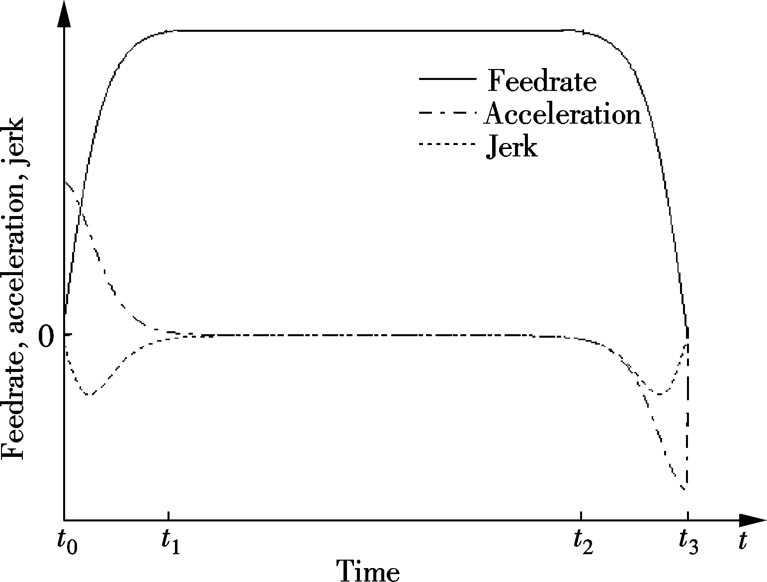
Fig.1 The kinetic model based on Sigmoid function

2.3 Constraint

In the kinetic model, the maximum value of feedratevmis codetermined by chord errorε, the radius of curvaturerand interpolator cycleT. Ref.[9] gave the constraint which is shown as

(7)

Given the assumption that the chord error and interpolator cycle is fixed, the greater the radius of curvature, the higher the upper limit of feedrate.

3 The Optimized Adams Algorithm

As mentioned in section 2, the new position parameteruj+1after one interpolator cycle should be computed in the interpolation process according to the current position parameterujand feedratev(t) in the path domain. This process is usually realized by the Taylor series expansion. The second-order Taylor expansion formula is shown as

(8)

According to the definition of instantaneous feedrate,

(9)

The shortcoming of Taylor series expansion is that the Taylor high-order expansion is necessary for high precision. It means that the higher order derivative of NURBS curveC(u) needs to be calculated. This is a very complicated process, but reducing the order of expansion will lower the precision. To resolve the problem, we present an optimized Adams-formula-based algorithm which can fasten theuj+1calculation.

The core concept of the Adams algorithm is to compute the current function value through the previousnsteps of the derivative values. The common Adams explicit formula is shown as

37y′(xn-2)-9y′(xn-3))

(10)

wherehis the stepping. The truncation error of this formula isO(t5)[10].

Applying this formula to interpolation, we can obtain

(11)

From Eq.(11), we know that the higher-order derivation can be avoided by using the Adams formula rather than the Taylor series expansion. However, there is still the first-order derivative in the formula. For this problem, we can replace the derivative with the difference quotient ofC(u).

(12)

Substituting Eqs.(12) and (9) into Eq.(11), we can obtain

(13)

For computing the position parameteruj+1, the previous several position parametersuj,uj-1,uj-2,… are needed, which means that this formula cannot be self-started. Other algorithms must be used to acquire the first several position parameters. The Eula formula or Runge-Kutta formula is the proper choice.

4 Computation of the Feed Value

After obtaining the position parameter in the parameter domainuj+1, the feed value in the path domain ΔX,ΔY,ΔZcan be computed. The steps of the feed value calculation are shown as follows.

4.1 Computing knot span of tool position

The NURBS curve is a type of piecewise parameter curve, so the first step is to determine the knot span in whichuj+1lies. We can use the linear or binary search to accomplish this task.

4.2 Computing nonzero basis function

From the De Boor-Cox recursion formula Eq.(2), we know that eachp-degree B-spline basis functionNi,p(u) is a linear combination of two (p-1)-degree basis functions. It means that we need to compute two product terms for one basis function. For example, assume thatp=2, 6 product terms need to be computed for 3 second-degree basis functions. 12 product terms need to be computed for 6 first-degree basis functions. That is to say, totally 18 product terms need to be computed for 3 second-degree basis functions, in which 9 kinds of low-degree basis functions are involved.

According to the property of the B-spline basis function, we know that in any given knot span [ui,ui+1), at mostp+1 basis functions are nonzero. They are namedNi-p,p,…,Ni,p. So we can draw the relation schema of each degree basis function. For example,N1,2,N2,2,N3,2are 3 second-degree basis functions that we want to compute. The nonzero basis function is in the solid box. From the schema we know that the first and the lastp+1 nonzero basis functions are only related to one low-degree nonzero basis function. As shown by the dotted arrows, there are a large number of low-degree zero-value basis functions. It is not necessary to calculate them (shown in the dotted box). Focusing on 3 second-degree basis functions again, actually 6 product terms (involving three types of low-degree basis functions) need to be computed. Based on Fig.2, the simplified algorithm is described as follows.

Assume that there arep+1p-degree nonzero B-spline basis functions,Ni-p+k,p(0≤k≤p), then

(14)

Fig.2 Relation schema of each degree basis

Ifk=0 ork=p,Ni-p+k,pis the first or lastp-degree B-spline basis function. When the degree changes frompto 0, the first and last basis functions in every degree are abided by the above principle. According to Eq.(14), the times of computing low-degree basis functionNi,pwill be effectively decreased. The times of computing low-degree basis function in different degrees through the classical De Boor-Cox algorithm and the simplified algorithm are compared in Tab.1.

Tab.1 Times of computing low-degree basis functions

4.3 Computing tool path coordinate

The NURBS curvesC(u) with weightwiand control pointsPican be obtained by substituting B-spline basis functionNi,p(u) computed by Eq.(14) into Eq.(1). According to the definition of parametric description, the coordinate value in the path domainX(uj+1),Y(uj+1),Z(uj+1) can be computed by

(15)

5 Simulation and Analysis

In order to verify the proposed algorithm, the experiments are simulated by Matlab. The parameters of NURBS curve are as follows:p=2; control points areP0(1,2),P1(1.5,1),P2(3,3),P3(4,3.5),P4(5,3),P5(6.5,1),P6(7,2); knot vectorU={0,0,0,1/5,2/5,3/5,4/5,1,1,1}; weightW={1,1,1,1,1,1,1}. The interpolator path is shown in Fig.3.

The machining parameters are given as follows: the interpolator cycleT=1 ms, the maximum value of feedratevm=4 mm/s, the initial feedratevs=0 mm/s, maximum chord errorε=1 μm. The feedrate can be computed through the kinetic model described by Eqs.(4) to (7). The feedrate-time profile is shown in Fig.4. Figs.3 and 4 show that the feedrate will slow down adaptively if the radius of curvature of tool path decreases. Fig.5 shows that the error is less than the maximum chord error and changes with the feedrate. From Eq.(13), the position para-

Fig.3 NURBS interpolator path

meteruand its stepping Δucan be computed. Their profiles are shown in Figs.6 and 7. These two figures indicate that the stepping of the parameter Δuwill also decrease if the radius of the curvature of the tool path reduces. Hence, the position parameter does not depend linearly on process time. Fig.8 shows that the jerk and the acceleration are continuous.

Fig.4 Feedrate profile

Fig.5 Error profile

Fig.8 Acceleration and jerk profile

The nonzero second-degree B-spline basis functionsNi,2can be computed based on Eq.(14). TheNi,2-uprofile is shown in Fig.9. Based on the computedNi,2, known weight and control points, the coordinate value in the path domainX(uj+1),Y(uj+1),Z(uj+1) can be computed by Eq.(15). According to these algorithms, the actual manufacture is tested by MD-3020 3d carving machine. The maximum cutting feedrate is 3 m/min. The speed of the main shaft is 2 000 r/min. The manufacture time is 2.54 s. The manufacture material is PVC. The manufacture process is shown in Fig.10.

Fig.9 The Ni,2-u profile

6 Conclusion

The whole process of the NURBS curves machining is designed based on the present algorithms. The modifications are presented in terms of feedrate planning, position

Fig.10 Manufacture processing

parameter computing and B-spline basis function calculation. Through the modified algorithms, the calculation times can be reduced, and the calculation speed can be increased while ensuring precision. Therefore, it is feasible to apply these algorithms to actual systems.

[1]Zhang Liyan, Bian Yuchao, Chen Hu, et al. Implementation of a CNC NURBS curve interpolator based on control of speed and precision [J].InternationalJournalofProductionResearch, 2009, 47(6):1505-1519.

[2]Sekar M, Narayanan V N, Yang S-H. Design of jerk bounded feedrate with ripple effect for adaptive NURBS interpolator [J].TheInternationalJournalofAdvancedManufacturingTechnology, 2008, 37(5/6):545-552.

[3]Peigl L, Tiller W.TheNURBSbook[M]. New York: Springer, 1995.

[4]Béarée R, Olabi A. Dissociated jerk-limited trajectory applied to time-varying vibration reduction [J].RoboticsandComputer-IntegratedManufacturing, 2013, 29(2):444-453.

[5]Lai J-Y, Lin K-Y, Tseng S-J. On the development of a parametric interpolator with confined chord error, feedrate, acceleration and jerk [J].TheInternationalJournalofAdvancedManufacturingTechnology, 2008, 37(1/2):104-121.

[6]Yong T, Narayanaswami R. A parametric interpolator with confined chord errors, acceleration and deceleration for NC machining [J].Computer-AidedDesign, 2003, 35(13):1249-1259.

[7]Liu X B, Ahmad F, Yamazaki K, et al. Adaptive interpolation scheme for NURBS curves with the integration of machining dynamics [J].InternationalJournalofMachineToolsandManufacture, 2005, 45(4):433-444.

[8]Du Daoshan, Liu Yadong, Yan Cunliang. An accurate adaptive parametric curve interpolator for NURBS curve interpolation [J].TheInternationalJournalofAdvancedManufacturingTechnology, 2007, 32(9/10):999-1008.

[9]Zhang Deli, Zhou Laishui. Intelligent NURBS interpolator based on the adaptive feedrate control [J].ChineseJournalofAeronautics, 2007, 20(5):469-474.

[10]Atkinson K, Han W M.Elementarynumericalanalysis[M]. Beijing: Post and Telecom Press, 2009.(in Chinese)

基于NURBS模型的自由曲线加工轨迹自适应生成方法

朱 昊1,2刘京南1杨安康1汪木兰2

(1东南大学自动化学院,南京210096)(2南京工程学院先进数控技术江苏省重点实验室,南京211167)

为实现NURBS曲面快速高精度实时差补,提出了基于修正型sigmoid函数的动力学模型,给出了最大速度、弓高误差、加工曲线的曲率半径和插补周期之间的约束条件.该模型在满足jerk、加速度、速度均连续的前提下,将常用的三次多项式S型以及三角多项式S型动力学模型的15个分段数减少至3个.在此基础上,提出采用差商代替导数的优化Adams算法,避免了常用的Taylor展开所遇到的高阶求导计算,求取了差补周期参数.最后通过减少低次零值B样条基函数的计算,对De Boor-Cox递推算法进行了简化设计,提出了精简型De Boor-Cox算法,缩减了计算量.仿真分析表明,所提算法可根据加工路径有效控制进给速度,在保证加工精度的同时,使计算量得到减少,提高了运算速度.实验结果显示本加工方法可以正确计算目标参数，并适合应用于实际加工系统.

自由曲线; NURBS; sigmoid函数; Adams算法

TP237

s：The Doctoral Fund of Ministry of Education of China (No. 20090092110052), the Natural Science Foundation of Higher Education Institutions of Jiangsu Province (No. 12KJA460002), College Industrialization Project of Jiangsu Province (No. JHB2012-21).

：Zhu Hao, Liu Jingnan, Yang Ankang, et al. An adaptive generation method for free curve trajectory based on NURBS[J]．Journal of Southeast University (English Edition),2014,30(3):296-301．

10.3969/j.issn.1003-7985.2014.03.007

10.3969/j.issn.1003-7985.2014.03.007

Received 2014-03-16.

Biographies：Zhu Hao(1980—), male, graduate, associate professor; Liu Jingnan(corresponding author), male, doctor, processor, liujn@seu.edu.cn.