Detached-eddy simulation of wing-tip vortex in the near field of NACA 0015 airfoil*
2014-06-01LIANGZhicheng梁志成
LIANG Zhi-cheng (梁志成)
Department of Engineering Mechanics, Shanghai Jiao Tong University, Shanghai 200240, China, E-mail: gassison.liang@gmail.com
XUE Lei-ping (薛雷平)
Department of Engineering Mechanics and MOE Key Laboratory of Hydrodynamics, Shanghai Jiao Tong University, Shanghai 200240, China
Detached-eddy simulation of wing-tip vortex in the near field of NACA 0015 airfoil*
LIANG Zhi-cheng (梁志成)
Department of Engineering Mechanics, Shanghai Jiao Tong University, Shanghai 200240, China, E-mail: gassison.liang@gmail.com
XUE Lei-ping (薛雷平)
Department of Engineering Mechanics and MOE Key Laboratory of Hydrodynamics, Shanghai Jiao Tong University, Shanghai 200240, China
(Received October 19, 2012, Revised January 14, 2013)
In the present study, the formation of the wing-tip vortex from a rectangular NACA0015 wing with a square tip at the Reynolds number of 1.8×10⁵and the angles of attack (AOA) α=8oand 10owere simulated with an incompressible detached eddy simulation (DES) method and the Reynolds averaged Navier-Stokes (RANS) equations with the SA model respectively. Numerical results were compared with experimental results to validate the capability of the employed methods in resolving tip vortex flows. The results show that DES model could capture the complicated three-dimensional structures in the vortex, and the streamwise vorticity and the cross-flow velocity agree with the experiment results quite well, but RANS-SA model with the same grid as that of DES failed to capture the correct structures and under-predicted the streamwise vorticity in the vortex by 40%. The present study suggests that under the same calculation cost, DES but not RANS-SA could be used to effectively predict the flow characteristics in tip vortex.
detached eddy simulation (DES), RANS-SA, wing-tip vortex
Introduction
The study of the near field of a wing-tip vortex could contribute to important applications both in hydrodynamics and aerodynamics. For example, the vortex generated by ship propellers may cause cavitations due to the low-pressure region in the core of the vortex, which often results in erosion damage and noise. Another one is the vortex shed from an aircraft wing may persist for some time after its generation, which is hazardous for other aircrafts going through it. However, the computational simulation of wing-tip vortex is a perplexing problem because of the presence of large gradients of velocity and pressure with high Reynolds numbersin the near field.
Therefore, the wing tip vortex has been widely studied experimentally and numerically in recent years. Birch et al.[1]measured the structure of tip vortexes in the near wake of a rectangular NACA 0015 airfoil with a square tip and a high-lift cambered air foil respectively using a seven-hole pressure probe with the Reynolds number of 2×10⁵. The structure of the tip vortex has been discussed from 0.5 to 2.5 chord length downstream of the leading edge. A wind tunnel experiment was performed by Ramaprian et al.[2], in which a three-dimensional laser Doppler velocimetry was used for measuring the three components of the instantaneous velocity to obtain the distributions of velocity, vorticity and circulation across the vortex at several axial locations. The experiment was also based on a rectangular square-tip NACA 0015 wing with the Reynolds number in the order of 105, which motivates the similar setup of the geometry and dynamic conditions for the numerical simulations in the present study. Other experiments have also been conducted to investigate the dynamics of the roll up of a tip vortex around the wing tip and its subsequent development in the near field[3-6].
As for numerical studies, flow around a three-dimensional bending hydrofoil was simulated by Xin et al.[7]using a RANS turbulence model with the commercial software Fluent. The numerical results were compared with experimental data obtained by the same research group. A discrepancy between the numerical and experimental results was found because the resolution of the grid for the vortex was not fine enough. Han et al.[8]simulated the flow in wing-tip vortex using the RANS model, in which different turbulence models had been tested. It was concluded that the RANS k-ω SST model was the most powerful one for the flows they had concerned with. Similar conclusions have been reached in other researchers’study[9]. An improved algebraic Reynolds stress model was also tested in Ye’s serial studies, which showed that the advantage of the improved model over other eddy-viscosity turbulence models was notable, but the pressure coefficient in the core of the vortex was still under-predicted by 11%. Ghisa et al.[10]and Li et al.[11]used LES. Besides, the tip vortexes shed from propellers were also studied by different researchers[12,13]. As for DES model, Mohamed et al.[14]compared the numerical results of DDES and RANS methods for a simulation of the wingtip vortex of NACA 0015 airfoil in dynamic stall condition, in which unstructured mesh was adopted. However, no experimental results were introduced for the validation.
Detached eddy simulation (DES), proposed in 1997, is a hybrid Reynolds averaged Navier-Stokes (RANS) / large eddy simulation (LES) model. It was designed to automatically turn to a RANS model in boundary layer and a LES model in separation regions. After being proposed, DES has been improved in recent decades[15-20]. Studies performed by many researchers showed that the accuracy of DES predictions for separation flows is superior to that of RANS[21,22], and at the same time, the cost of DES is less than that of LES.
The objective of this study is to test the capability of DES of simulating the flow in wingtip vortex. In this paper, the near-field characteristics of wing-tip vortex of NACA 0015 airfoil at α=8oand 10oare investigated with both the DES model and the RANSSA model. The results of these cases are compared to experiments[1,2].
1. Numerical procedure
1.1 Turbulence modeling
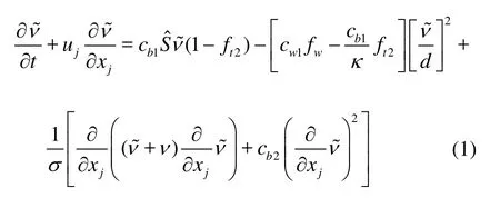
The unsteady turbulent flow was modeled by the Naiver-Stokes (N-S) equations, in which the turbulence effects were taken into account via an eddy viscosity approach. In this paper, the DES based on the SA model was adopted. The SA model is a one-equation turbulence model. It solves a transport equation of turbulent eddy viscosity ν~. The transport equation reads
In Eq.(1), ν~ is the turbulence viscosity, and d is the wall distance. The model variables and constants in Eq.(1) were carefully described in Ref.[23].
The switch between RANS and LES in the original DES-SA model was achieved by replacing the explicit length scale d, the wall distance, with a blending function l~ involving d and the length scale of the grid size as
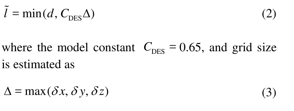
in which δx, δy, δz represent the grid sizes in three dimensions respectively.
For the flow close to the wall, where d<CDESΔ, the original RANS model was employed. And LESSGS model was used for the flow away from the wall, where d>CDESΔ.
Spalart et al.[17]introduced a “delay” effect to the original DES-SA model by modifying the blending function from one only depending on grid to one also depending on eddy-viscosity field. The improved DES model was addressed as Delay-DES (DDES for short). The expression “delay” means delaying the DES model turning into its LES branch.
The blending function of (3) is replaced by
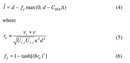
where fdwas designed to be 1 in the LES region, where rd≤1, and 0 elsewhere. So according to (4), inthe RANS region, fdwill be set to 0, while setting fdto 1 will turn the model to the original DES model. More details about DDES can be found in the Ref.[17]. In the current paper, the DDES model is applied.
1.2 Numerical method
The simulations presented in the present study were carried out using the open-source code OpenFOAM. The flow was assumed incompressible. A cell-centered finite volume method was adopted. Gradient terms of the N-S equations were discretized using a second-order central differencing scheme. The second order implicit backward differencing in time was applied. The PISO algorithm was used to enforce pressure/velocity coupling.
1.3 Mesh and flow configuration
Simulations of the NACA0015 airfoil flows in the tip vortex region at the angles of attack 8oand 10owas carried out to validate the capability of RANS-SA and DDES. The Reynolds number of Re=1.8×10⁵was used for the comparison with the experiment[1,2].
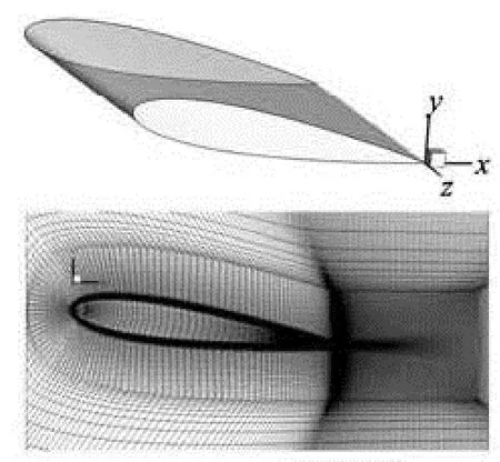
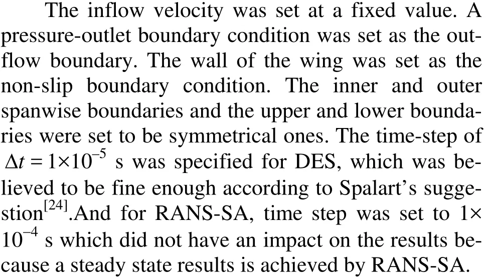
The computational model of the wing and the mesh at the wing tip in the x-y plane is shown in Fig.1. The origin of the coordinate system (x for streamwise, y for vertically upward, and z for spanwise) is at the tip of the trailing edge.The first step near the wall+
y was set to be less than 1, which was fine enough for the SA model according to Spalart’s suggestion[24]for DES grid design. The grid where tip vortex would be generated was refined up to 0.6 chord length downstream of the trailing edge. The grid in the near field was close to cubic because it should be in the LES region. The upstream boundary was three chord lengths away from the leading edge. The upper and lower boundaries were four chord lengths away from the wing surface. The outflow boundary was located at five chord lengths downstream of the trailing edge. The span length of the airfoil was one chord with one end fixed to the symmetry wall and the other exposed in the flow to generate a tip vortex. One chord length space was left from the wing tip to the flow field boundary. The total number of grids is more than 4×10⁶.
2. Results and discussion
The mean field, obtained by the average over 30 non-dimensional time (normalized by chord length c and the free-stream velocity tU∞/c period after the flow being fully developed, was used to illustrate the flow structure of the tip vortex as well as to be compared with the experimental data[1,2], for the validation of the capability of DES and RANS-SA model. It should be noted that the mesh, numerical scheme, and other configurations of DES and RANS were kept the same except the difference in time step mentioned in Section 1. Numerical data were collected and plotted according to the experimental results.
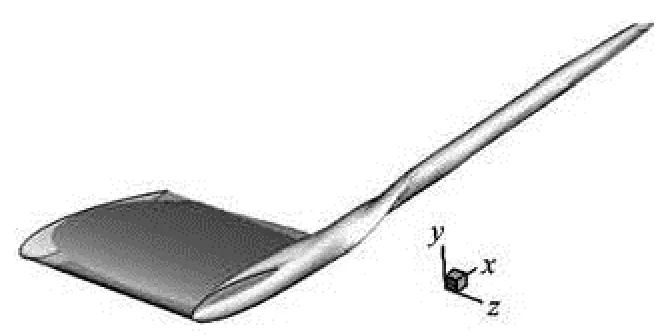
Fig.2 Instantaneous iso-surfaces of normalized streamwise vorticity ωxc/2U∞=7.5, simulated by DES, AOA=10o
2.1 NACA 0015 α=10o
Figure 2 shows the instantaneous iso-surfaces of normalized streamwise vorticity ωxc/2U∞=7.5. From the three-dimensional vortex topology in the formation region, at least two obvious strong vortex systems could be observed. These two vortex systems started to wrap each other from x/ c≈–1.5. The shape of the tip vortex presents non-axisymmetry because of the vortices interaction. At about one chord length downstream, the vortex system became axisymmetrical. The structures of two-vortex systems agree with the experimental results[1]and LES results[10]well. In Fig.3, contours of non-dimensional streamwise vorticity were plotted at different streamwise positions(x/ c=-0.5, -0.25, -0.1), and compared with the experimental results[1].
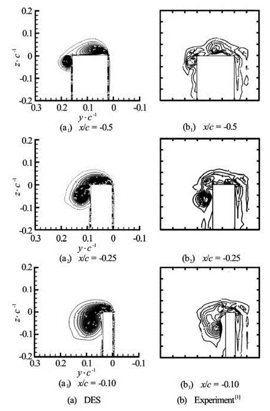
Fig.3 Time-averaged contours of normalized streamwise vorticity ωxc/2U∞at different streamwise positions (x/ c= -0.5, -0.25, -0.1), numerical results and experimental results
Figure 4 shows normalized the streamwise vorticity at x/ c=0.33. It should be noticed that the vorticity was normalized by ωxc/ U∞instead of ωxc / 2U∞. The difference is due to the fact that the contours are from different experiments. Both DES and RANS-SA results are plotted to be compared with the experiment[2]. The non-axisymmetrical structure vortex has been captured by both DES and RANS. The maximum magnitude simulated by DES reaches 20, which agrees quite well with the experimental result[2]. But the RANS-SA model predicted a maximum magnitude of 15, which is less than the experimental result by 25%. Besides, it can be clearly observed that in the vortex core, the result of streamwise vorticity gradient with DES is larger than that with RANS-SA, and DES has captured one more peak of streamwise vorticity magnitude in the core, which reflects the interaction of main and secondary vortices. In contrast, RANS-SA just got a large area of the peak. This shows the capability of DES in capturing the small spatial structure in the vortex, while RANS-SA model could just capture the general structure.
Fig.4 Contours of normalized streamwise vorticity ωxc/ U∞at x/ c=0.33, numerical results and experimental results
Figure 5 gives the contours of normalized streamwise velocity Ux/U∞at x/ c=0.33. The axial component of velocity field within the vortex is highly three-dimensional at x/ c=0.33 because of the roll up process near the trailing edge. The structure of the distribution has been captured by DES agreeing with experimental results[2]. However, the difference between numerical results and experiments is also obvious. In experiments, the normalized streamwise velocity generally decreases from 1 at the edge of the vortex to 0.68 at the center, but in the DES results, the value decreases from 1 along the reversed radial dire-ction, and at some position in the vortex, the value reaches a minimum value 0.83, and at the center of the core, the value recovers to 0.91. This kind of distribution of streamwise velocity is generated by the spiral movement in the vortex. More details could be found in the case of α=8o. In contrast, the RANS-SA model failed to get the complex structure in the vortex.
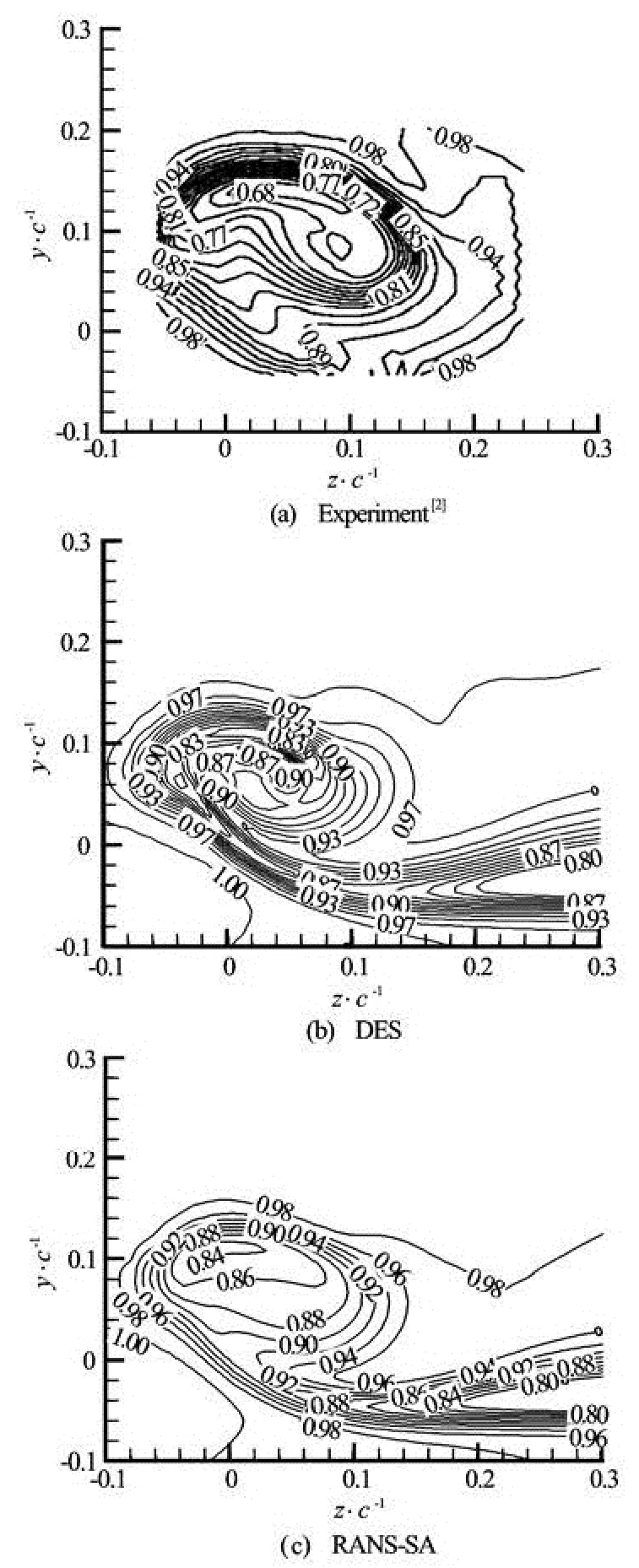
Fig.5 Contours of normalized streamwise velocity ωxc/ U∞at x/ c=0.33, numerical results and experimental results
2.2 NACA 0015 α=8o
The case of 8oangle of attack has been simulated by DES and RANS-SA using the same grid. The results were compared with the experiment[1]as discussed blow.
Figure 6 shows the magnitude of streamwise vorticity normalized by ωxc/ U∞at the cross-flow plane of x/ c=0.5. The comparison between DES and experiments shows that the results of DES agree with the experiments quite well in terms of the peak value of streamwise vorticity magnitude and the width of the vortex. And DES has captured even smaller structures in the vortex, which might be due to the fact that the grid of experiments was not fine enough. In contrast, RANS-SA has under-predicted the peak value by 40%.
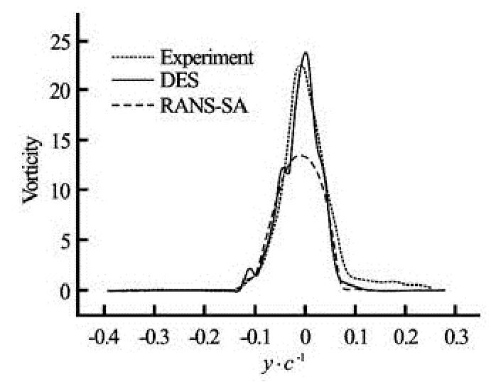
Fig.6 Magnitude of normalized streamwise vorticity ωxc/ U∞in tip vortex at a cross-flow plane of x/ c=0.5, comparison between DES, RANS-SA and experiment[1]
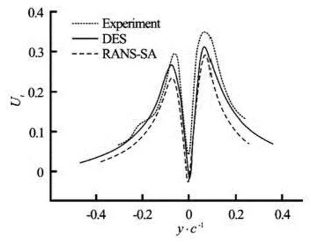
Fig.7 Magnitude of normalized tangential component of velocity Ut=/U∞in tip vortex at a cross-flow plane of x/ c=0.5, comparison between DES, RANS-SA and experiments[1]

Fig.8 normalized streamwise component of velocity Ux=u/ U∞in tip vortex at a cross-flow plane of x/ c=0.5, comparison between DES, RANS-SA and experiment[1]
Figure 7 shows the magnitude of normalized tangential component of velocity Ut=/U∞in the tip vortex in the cross-flow plane of x/ c=0.5. It could be observed that both DES and RANS-SA have under-predicted the peak value of tangential velocity. But the result given by DES is still better than that of RANS-SA.
Figure 8 shows the normalized streamwise component of velocity Ux=u/ U∞in the tip vortex at x/ c=0.5. The recovery of streamwise velocity in the core of the vortex (the same kind of structure is also shown in Fig.6) has been captured by both DES and experiment[1]. This complex structure was generated by the rolling up movement in the vortex.
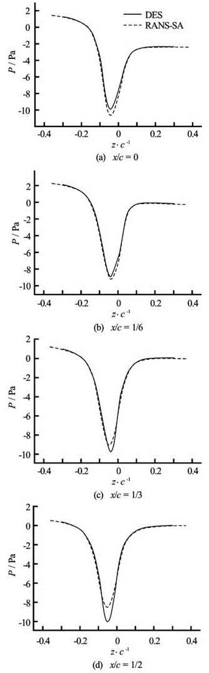
Fig.10 Pressure distribution in the tip-vortex at different crossflow planes (x/ c=0, 1/6, 1/3, 1/2)
A detailed development process can be observed in Fig.9, where DES has captured the correct wrapping structure inside the vortex. On the other hand, at x/ c=0, which is set as the trailing edge of the wing, the RANS-SA results are similar to those of DESbecause near the wall, DES is in its RANS bench. At even downstream location (x=1/6, 1/3, 1/2), DES has captured the small streamwise velocity structure because of the spiral in the vortex, but RANS-SA did not. It should be also noticed that both DES and RANS-SA have captured a decrease of streamwise velocity which was not captured by experiments in vortex at about y/ c=–0.1. The decrease is illustrated by Fig.9, in which the arrow showed the position of the small structure. The reason why the experiment has not captured the decrease might be that the grid of experiment was not fine enough in this region.
Figure 10 shows the results of DES and RANSSA about the pressure in the tip-vortex. It could be found that at x/ c=0 and x/ c=16, the pressure drop got by different methods are very close, but at x/ c= 1/3, RANS-SA results begin to be smaller than DES results, and the difference is very obvious at x=1/2. The difference between DES and RANS-SA could explain why minimum pressure along the tip vortex core is always under-predicted. The reason is not just because of the coarse grid, and the RANS-SA model itself might meet difficulty when dealing with wing-tip vortex flows.
3. Conclusions
In this paper, wing-tip vortex flows have been simulated by the DES and RANS-SA models to validate the capability of different methods in predicting this kind of flows. The results got by DES and RANSSA have been compared with each other and with experimental results[1,2]. Only averaged results are compared because no transient data are available in the experiment results. However, transient analysis such as velocity fluctuation is one of the advantages of DES. Further work will be performed to study the transient characteristics of wing-tip flows by DES in the future.
The results indicate that DES could capture complex three-dimensional structures in the vortex, and the streamwise vorticity as well as the cross-flow velocity agree quantitatively with the experiment results. But the RANS-SA model, with the same grid as that of DES, has failed to capture the correct structure in the vortex flows, and under-predicts the vorticity in tip vortex by 40%. The minimum pressure in vortex got by RANS-SA is larger than that of DES downstream of the wing tip, which could be attributed to the stronger effects of vortex dissipation in the RANS-SA simulation. All the results show that the DES-SA model could simulate the flow characteristics in tip vortex effectively, where the RANS-SA model always meet difficulties.
[1] BIRCH D., LEE T. and MOKHTARIAN F. et al. Structure and induced drag of a tip vortex[J].Journal ofAircraft,2004, 41(5): 1138-1145.
[2] RAMAPRIAN B. R., ZHENG Y. X. Measurements in rollup region of the tip vortex from a rectangular wing[J].AIAA Journal,1997, 35(12): 1837-1843.
[3] IGARASHI H., DURBIN P. A. and MA H. et al. A Stereoscopic PIV study of a near-field wingtip vortex[R]. AIAA Paper 2010-1029, 2010.
[4] GU Yun-song, CHENG Ke-ming and ZHENG Xin-jun. Flow field characteristics of wing tips vortex and its control[J].Acta Aerodynamics Sinica,2008, 26(4): 446-451(in Chinese)
[5] LI Guang-nian, ZHANG Jun and ZHANG Guo-ping et al. Propeller wake analysis by means of PIV in large water tunnel[J].Acta Aerodynamics Sinica,2010, 28(5): 503-508(in Chinese)
[6] DEL PINO C., LOPEZ-ALONSO J. M. and PARRAS L. et al. Dynamic of the wing-tip vortex in the near field of a NACA0012 airfoil[J].Aeronautical Journal,2011, 115(1166): 229-240.
[7] XIN Gong-zheng, LU Lin-zhang and LIU Deng-cheng et al. Experimental and numerical study of the velocity field in the tip vortex of a 3D bending hydrofoils[C].Proceedings of the 9th National Congress on Hydrodynamics and 22nd National Conference on Hydro-dynamics.Chengdu, China, 2009, 438-447(in Chinese).
[8] HAN Bao-yu, XIONG Ying and YE Jin-ming. Effect of turbulence models on numerical simulation of tip vortex flow field behind 3D wing[J].Acta Aeronautica et Astronaut ICA Sinica,2010, 31(12): 2342-2347(in Chinese).
[9] FLASZYNSKI P., SZANTYR J. A. and BIERNACKI R. et al. A method for the accurate numerical prediction of the tip vortices shed from hydrofoils[J].Polish Mari-time Research,2010, 17(2): 10-17.
[10] GHISA R., MITTAL R. and DONG H. Study of tipvortex formation using large-eddy simulation[R]. AIAA Paper 2005-1280, 2005.
[11] LI Jiang, CAI Jian-gang and LIU Chao-qun. LES for near field wakes behind junction of wing and plate[J].Journal of Hydrodunamics, Ser. B,2006, 18(3Suppl.): 270-274.
[12] YE Jin-ming, XIONG Ying and SHENG Li. Numerical computation method of propeller tip-vortex roll-up[J].Journal of Naval University of Engineering,2007, 19(6): 58-66(in Chinese).
[13] HONG Fang-wen and DONG Shi-tang. Numerical simulation of the structure of propeller’s tip vortex and wake[J].JournalofHydrodynamics,2010, 22(5Suppl.): 457-461.
[14] MOHAMED K., NADARAJAH S. and PARASCHINOIU M. Detached eddy simulation of a wing tip vortex at dynamic stall conditions[J].Journal of Aircraft,2009, 46(4): 1302-1313.
[15] TRAVIN A., SHUR M. and STRELETS M. et al. Detached-eddy simulation past a circular cylinder[J].Flow,Turbulence and Combustion,2000, 63(1-4): 293-313.
[16] MCCALLEN R., BROWAND F. and ROSS J.The aerodynamics of heavy vehicles: Trucks, buses and trains[M]. Berlin, Heidelberg, Germany: Springer- Verlay, 2004, 339-352.
[17] SPALART P. R., DECK S. and SHUR M. et al. A new version of detached-eddy simulation, resistant to ambiguous grid densities[J].Theoretical ComputationalFluid Dynamics,2006, 20(3): 181-195.
[18] SHUR M. L., SPALART P. R. and STRELETS M. K.et al. A hybrid RANS-LES approach with delayed DES and wall-modeled LES capabilities[J].International Journal of Heat and Fluid Flow,2008, 29(6): 1638- 1649.
[19] NIKITIN N., NICOUD F. and WASISTHO B. et al. An approach to wall modeling in large-eddy simulations[J].Physics of Fluids,2000, 12(7): 1629-1632.
[20] TRAVIN A., SHUR M. and STRELETS M. Physical and numerical upgrades in the detached-eddy simulation of complex turbulent flows[J].Fluid Mechanics and its Applications,2004, 65: 239-254.
[21] STRELETS M. Detached eddy simulation of massively separated flows[R]. AIAA Paper 2001- 0879, 2001.
[22] SPALART P. R. Detached-eddy simulation[J].AnnualReview Fluid Mechanics,2009, 41: 181-202.
[23] SPALART P. R., ALLMARAS S. R. A One-equation turbulence model for aerodynamic flows[J].La Reche-rche Aerospatiale,1994, 1(1): 5-21.
[24] SPALART P. R. Young Person’s guide to detachededdy simulation grids[R]. NASA Contractor Report, NASA/CR-2001-211032, 2001.
10.1016/S1001-6058(14)60022-6
* Project supported by the National Natural Science Foundation of China (Grant No. 11102110).
Biography: LIANG Zhi-cheng (1988-), Male, Master
XUE Lei-ping, E-mail: lpxue@sjtu.edu.cn
猜你喜欢
杂志排行

水动力学研究与进展 B辑的其它文章
- The analysis of second-order sloshing resonance in a 3-D tank*
- Comprehensive analysis on the sediment siltation in the upper reach of the deepwater navigation channel in the Yangtze Estuary*
- Two-phase air-water flows: Scale effects in physical modeling*
- Numerical prediction of 3-D periodic flow unsteadiness in a centrifugal pump under part-load condition*
- Effect of compressive stress on the dispersion relation of the flexural–gravity waves in a two-layer fluid with a uniform current*
- Capillary effect on the sloshing of a fluid in a rectangular tank submitted to sinusoidal vertical dynamical excitation*