Modelling of 2-D extended Boussinesq equations using a hybrid numerical scheme*

FANG Ke-zhao (房克照), ZHANG Zhe (张哲), ZOU Zhi-li (邹志利), LIU Zhong-bo (刘忠波)

State Key Laboratory of Coastal and Offshore Engineering, Dalian University of Technology, Dalian 116024, China

National Marine Environment Monitoring Center, State Oceanic Administration, Dalian 116023, China, E-mail: kfang@dlut.edu.cn

SUN Jia-wen (孙家文)

National Marine Environment Monitoring Center, State Oceanic Administration, Dalian 116023, China

Modelling of 2-D extended Boussinesq equations using a hybrid numerical scheme*

FANG Ke-zhao (房克照), ZHANG Zhe (张哲), ZOU Zhi-li (邹志利), LIU Zhong-bo (刘忠波)

State Key Laboratory of Coastal and Offshore Engineering, Dalian University of Technology, Dalian 116024, China

National Marine Environment Monitoring Center, State Oceanic Administration, Dalian 116023, China, E-mail: kfang@dlut.edu.cn

SUN Jia-wen (孙家文)

National Marine Environment Monitoring Center, State Oceanic Administration, Dalian 116023, China

(Received January 5, 2013, Revised March 28, 2013)

In this paper, a hybrid finite-difference and finite-volume numerical scheme is developed to solve the 2-D Boussinesq equations. The governing equations are the extended version of Madsen and Sorensen’s formulations. The governing equations are firstly rearranged into a conservative form. The finite volume method with the HLLC Riemann solver is used to discretize the flux term while the remaining terms are discretized by using the finite difference method. The fourth order MUSCL-TVD scheme is employed to reconstruct the variables at the left and right states of the cell interface. The time marching is performed by using the explicit second-order MUSCL-Hancock scheme with the adaptive time step. The developed model is validated against various experimental measurements for wave propagation, breaking and runup on three dimensional bathymetries.

hybrid scheme, Boussinesq equations, TVD, Riemann solver

Introduction

The accurate prediction of the water wave propagation is of fundamental and practical importance to marine and coastal engineering. Over the last decades, the Boussinesq equations were widely used to describe the wave transformation in the coastal region and are well known as the most state-of-the-art coastal wave models[1]. The success of the Boussinesq models is mainly due to the stable and efficient numerical implementation, in addition to the enrichment of Boussinesq wave theories and the development of modern computer technology.

Though the finite element method (FEM)[2]and the spectral method[3]can also be used to solve Boussinesq equations, in the existing numerical approaches, the Finite Difference Method (FDM)is mainly adopted. The simple method proposed by Wei and Kirby[4]for solving the fully nonlinear equations is among the existing numerical approaches. In order to ensure that the truncation error of the numerical scheme is less than that of the dispersion embodied in the governing equations, in this scheme all the first-order spatial derivatives are approximated by using fourthorder accurate finite differences while the secondorder accurate differences are used for third spatial derivatives. The time marching is performed by using a third-order Adams-Bashforth predictor and a fourthorder Adams-Moulton corrector, that is iterated until the convergence is achieved. This numerical scheme is shown to be accurate and efficient, and followed extensively in the subsequent researches[5,6].

However the improvements to the FDM-solver based models are required to develop a more user-friendly and operational model. Firstly, the models tend to be noisy or at least weakly unstable to high wavenumbers near the grid Nyquist limit[7]. Numerical filters are usually used sparsely to stabilize the models. Though they work well in some cases, the use of artificial numerical filters on real flow phenomena is unavoidably involved. In addition, the wave breaking andthe moving wet-dry interface in Boussinesq models are treated empirically, which are characterized by many tunable parameters. This on one hand introduces an additional noisy source and on the other hand brings some uncertainty to the computed results.

The above shortages can be overcome by using a hybrid finite-volume and finite-difference method in the numerical solution of Boussinesq equations, as shown very recently in Refs.[7-16]. The main feature of the hybrid numerical scheme is summarized as follows. The Boussinesq formulations are firstly written in the conservative forms. Then the Finite Volume Method (FVM) is used to discretize the convective flux terms while the rest terms are approximated by using the FDM. The implementation of the FVM usually includes the use of a higher resolution method with the shock-capturing ability to be borrowed directly from the numerical schemes for hyperbolic conservative laws[17]. Once the wave breaking or the wetdry interface occurs, Boussinesq equations are turned into nonlinear shallow water equations(NLSW) by switching off higher order nonlinear and dispersive terms. In this way, the wave breaking and the wet-dry interface are treated as the bore and the local Riemann problem, respectively, in the NLSW and embodied in the high-resolution FVM scheme automatically. The aforementioned results from the hybrid numerical scheme are shown to be great improvements over the traditional FDM solver.

However, it is known that the existing hybrid numerical solvers are mainly limited to one-dimensional problem except in the work of Shi et al.[7], Tonelli and Petti[14]and Roeber and Cheung[16]. The objective of this study is to extend the hybrid FVM/FDM scheme to two dimensional Boussinesq equations with a further investigation of the wave propagation over complex three-dimensional bathymetries. The governing equations adopted here are the two-dimensional extended Boussinesq equations recently derived by Kim et al.[18], where the Madsen and Sorensen’s formulations[19]are extended by including higher order bottom curvature terms. The mathematical model is presented in Section 2. The numerical implementation is described in Section 3. The numerical tests are conducted in Section 4 and the final conclusions are in the last Section.

1. Boussinesq type equations

1.1 Boussinesq equations for rapidly varying bathymetry

The 2-D extended Boussinesq equations are in the forms[18]

where η is the surface elevation, d=(h+η) is the total water depth, h is the still water depth, P and Q are the velocity flux components in x and y directions, respectively. The subscripts x, y, t denote the partial derivatives with respect to x, y and time.xψ andyψ are the dispersive terms expressed by

where B is the dispersion parameter, B=1/15 in the Pade [2,2] approximation of the exact linear dispersion relation. Neglecting higher order terms related to the seabed (the last three terms in Eqs.(4) and (5)), the equations are returned to the Madsen and Sorensen’s equations[19]. Including these terms helps to improve the model’s performance for rapidly varying bathymetry[18].

To facilitate the FVM implementation of the governing equations, the source terms gdηxand gdηyare reformulated into the form as

which are well-balanced for the unforced, still water condition[7,15].

1.2 Conservative form of Boussinesq-type equations

The governing equations are written in the conservative form

where U is the variable vector, F( U) and G( U) are the flux vector along x and y directions, respectively, S( U) is the source term. The expressions for these variables are

In Eq.(8), U and V are the sum of the terms related to the time derivatives and defined as

In Eq.(10), the x and y components of the dispersive terms φ are listed as

τ in Eq.(10) is introduced to account for the bottom friction, whose two components are[13]

f is the friction coefficient and typically in the range of 0.001-0.01. In the present study, f serves as a tunable parameter and is determined by matching the numerical results to the measurements. The optimum value of f will be clearly illustrated in Section 3 for each simulation test, otherwise the bottom friction is not included.

2. Hybrid numerical scheme

2.1 Spatial discretization

The computational domain is discretized by using rectangular cells indexed as xi=iΔx( i= 1,…M) and yj=jΔy( j=1,…N) (M and N are the gird numbers in x and y directions, respectively). The governing equations are integrated for the (i, j)th cell over the bounded finite volume [xi-1/2,xi +1/2]× [yj-1/2,yj +1/2]and with the use of the Green theorem, the explicit updating formula is obtainedwhere the superscript n denotes the time level, Δt is the time step,is redefined as the average variables of a cell volume. Fi-1/2,jand Fi+1/2,jrepresent the fluxes through the left- and right-cell interfaces, while Gi, j-1/2and Gi, j+1/2are the fluxes through the south and north cell interfaces, respectively. Si, jis the numerical source for the cell (i, j).

A hybrid finite-difference and finite-volume method is used to spatially discretize the governing equations. The convective flux terms are approximated by using the FVM while the rest terms are approximated by using the FDM.

2.1.1 Finite volume implementation of convective flux

The HLLC approximate Riemann solver is adopted to evaluate the interface flux Fi+1/2,jas[17]

in which FL=F( UL), FR=F( UR), subscripts L and R representing the left and right Riemann states of a local Riemann problem, as shown in Fig.1. F*Land F*Rare the numerical fluxes in the left and right parts of the middle region of the Riemann solution and expressed as

Fig.1 The sketch of local Riemann problem

where subscripts 1 and 2 are used to define the first and second components of the flux vector F, and vLand vRare the left and right initial values of a local Riemann problem for the tangential velocity component. F*is calculated by using the HLL formula given by Harten et al.[20]

In order to apply the HLL flux properly to the shallow water equations, it is important to identify the correct wave speeds SL, SRand SM. Toro recommended the use of a two-rarefaction approximate Riemann solver for SLand SR[17]. The wave speed estimates under this assumption are

As to the middle wave speed SM, Toro suggested that the following choice is most suitable for dry-bed problems[17]

Fig.2 Experiment setup and measurement transects in the experiments by Berkhoff et al.[21]

Fig.3 Comparisons of numerical results and experimental data on different transects

2.1.2 Finite difference implementation of the remaining terms

Following Orszaghova[15], the source term S in Eq.(16) is discretized by using the finite difference method. The implementation is simple and will not be repeated here.

After the time integration, the independent values of P and Q need to be evaluated from Eqs.(11) and (12). The derivatives in Eq.(11) are approximated by using the second-order finite difference formula and the Q related quantities are put to the right hand side of the equation (this helps the use of the adaptive time step for the time integration[7]). Finally a tri-diagonal matrix system with M unknowns for each jth row is formed and could be solved by using a Thomas algorithm efficiently. The scheme is also extended to Eq.(12) in a similar way.

2.2 Time marching scheme

The integration of the governing equations through time is achieved by the MUSCL-Hancock scheme, which is a second-order Godunov-type and involves a two-stage predictor/corrector method. The predictor is marched to a half time step forward from the time layer n

The flux term is then evaluated by using the predicted variables, the corrector step over one time step is given by

The time step Δt is time-varying and dependent upon the CFL condition

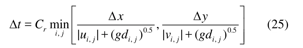
where Cris the Courant number, and is set to 0.5 in all simulations to ensure that the CFL condition is always maintained.

Fig.4 The instantaneous surface elevations from the simulation

Fig.5 Wave amplitude for the first-, second- and third-harmonics along the center line

2.3 Boundary conditions and wave breaking

Three ghost cells are set around the entire computational domain, the cell number is determined by the combination need of the MUSCL and finite difference formulas. For a solid reflective boundary along x direction, we set

And it could be extended to the y direction in a similar way.

Fig.6 Schematic diagram of the conical island laboratory experiment

Fig.7 Wave transformation around the conical island for A/ h=0.096

The ratio of the free surface elevation to the water depth is adopted as the criterion to switching off the Boussinesq terms, which is set to 0.8 according to previous experiences[7,14]. To capture the wet-dry interface accurately, the wave speed in Eq.(20a) and Eq.(20b) should be corrected aswhere a minimum water depth (=0.0001m) is used to mark the cells with dry or wet state.

Fig.8 Time series of free surface elevation for solitary wave transformation around the conical island (left): A/ h=0.045, (right): A/ h=0.096

Following the FUNWAVE model[5], the incident waves are generated internally in the computational domain by adding a source function to the mass equations. A sponger layer function (in the form of 2 tanh() with values varying smoothly from 0 to 1 is multiplied to the numerical solutions at each time step to absorb the wave energy if necessary.

3. Numerical results and discussions

Numerical simulations are conducted in this section to validate the developed model, including (1) monochromatic wave propagation over a submerged elliptical shoal on a slope, (2) nonlinear refraction-diffraction of regular waves over a semicircular shoal, (3) solitary wave runup on a conical island, (4) solitary wave transformation over a three dimensional reef with a conical island. The first two cases do not involve a wet-drying boundary and are used to demonstra-te model’s capability in describing the nonbreaking and dispersive wave transformation over complex three-dimensional bathymetries. The third case is chosen to test model’s capability in capturing the wetdry interface. The fourth case is the most critical test because it involves both the wave breaking and the time-varying wet-dry interface. It is also worth noting that no additional numerical filter is used for all simulations presented, demonstrating that the developed model is stability-preserving.

3.1 Wave propagation over an elliptical shoal

Berkhoff et al.[21]conducted laboratory experiments of the monochromatic wave propagation over a submerged elliptical shoal on a slope, which serves as a standard test for verifying nonlinear dispersive wave models. The experimental geometry and the measurement transects are shown in Fig.2. The water depth at the wave maker (x=0 m) is 0.4572 m and the incident monochromatic wave has a period of 1.0 s and an amplitude of 0.0232 m.

In the simulation, the computational domain is modified by extending the domain from x=0 m to -3.0 m with a constant wave depth of 0.45 m and from x=25.0 m to 28.0 m with a constant wave depth of 0.07 m. The extended domain is discretized into numerous cells each of a size of Δx=0.05 m and Δy =0.10 m. The internal source for generating the corresponding monochromatic waves is located at x=0 m. Two sponge layers of 2 m and 3 m in width are placed behind the wave maker and at the end of the beach to absorb the wave energy. The model is run for 40 s. The computed wave height at eight measurement transects are compared against the experimental data in Fig.3. The agreements are generally good, demonstrating that the present numerical model can accurately simulate the combined effects of the wave shoaling, the refraction, the diffraction, and the reflection, as involved in this test.

3.2 Non-linear refraction-diffraction of regular waves over a semicircular shoal

Whalin experimentally studied the propagation of regular waves over a semicircular shoal , which is the classical problem for verifying nonlinear and disperseve wave models[2]. Here we concentrate on the case with a wave period of 2 s and a wave amplitude of 0.0075 m. The computational domain is discretized into 601 cells in x direction and 81 cells in y direction, each of a size of 0.0762 m×0.0762 m. The source for generating the corresponding incident wave is located at x=6.0 m. The sponger layer with a length of 5 m is placed behind the wave maker and at the downstream boundary to absorb the wave energy.

An instantaneous surface elevation field obtained from the model is shown in Fig.4, where the focusing of the incident linear waves over the semicircular shoal is clearly illustrated. The shoaling and focusing process involves the energy transfer from the primary frequency to high harmonics. The spatial variation of the first-, second- and third-harmonics from the computation is compared with the experimental data in Fig.5. The numerical results from the FDM method[19]and the FEM method[2]for the problem are also presented for comparison. The numerical results from three numerical models are almost identical except for a slight difference in the first- and second- harmonics after x=20 m, and they all are in good agreements with the experimental data. The accuracy of the proposed numerical scheme is thus confirmed. Though achieving the same level of accuracy, the proposed hybrid scheme is more cost-effective than the FEM method and more stable than the FDM method.

Fig.9 Maximum inundation around the conical island

Fig.10 Bathymetry contours and measurement locations for swigler experiments[23]

Fig.11 Snapshots of solitary wave transformations over three-dimensional reef

3.3 Solitary wave runup on a conical island

It is shown that the refraction and the diffraction of tsunami waves may result in a significant inundation on the lee side and the trapping of energy around an isolated island[22]. Briggs et al. experimentally studied this problem by investigating the solitary wave runup on a conical island[22]and the collected data are widely used for verifying runup models.

Figure 6 shows the schematic diagram of the experiment. The basin is 25 m long and 30m wide. The circular island has the shape of a truncated cone with a diameter of 7.2 m at the bottom and 2.2 m at the top. The height of the conical island is 0.625 m and has a side slope of 1:4. The wave maker is 27.4 m long and it generates the solitary waves for the laboratory test. The wave absorbers at the three remaining sidewalls are used to reduce the reflection.

The present study considers a smaller water depth h=0.32 m from the experiments and two initial solitary wave heights A/ h=0.045, 0.096. In the simulation, we let Δx=Δy=0.10 m, and the friction coefficient f=0.005. The computational domain is primarily the same as the experimental setup but is modified by extending the domain from x=0 m to -10.0 m with a constant water depth of 0.32 m in order to use a solitary wave solution as the initial condition. A series of snapshots for the initial solitary wave with A/ h=0.096 are shown in Fig.7. The main physical process involved are reproduced by the model, such as the maximum runup at the front (t= 29.3 s), the refraction and the trapping of the solitary wave over the island slope (t=31.4s), the maximum runup on the leeside of the island due to the superposition of diffracted waves and trapped waves (t= 33.3 s) and the rundown and the subsequent propagation of waves behind the island (t=34.0s).

The computed time series of the surface elevations are compared against the experimental data in Fig.8 at six measurement locations for two cases. These gauges play an important role in the experiment for the reason that they provide a sufficient coverage ofthe wave conditions. The overall agreements are good. The model accurately captures the main stroke from the solitary wave but fails to reproduce the small amplitude shore period waves afterwards, which is inconsistent with the most published shallow water models. The calculated runup from the model is compared against the experimental data in Fig.9. They are in close agreements, demonstrating that the model could accurately simulate the wet-dry interface.

Fig.12 The comparison of time series of free surface elevation between the model and experimental data

3.4 Solitary wave transformation over a three-dimensional reef

Swigler conducted laboratory experiments for solitary wave transformation over a three-dimensional reef with a conical island in a large wave basin at Oregon State University’s O. H. Hinsdale Wave Research Laboratory[23]. Compared with the previous tests, this test is critical as the wave breaking and the time-dependent wet-drying interface are involved. The sketch of the wave basin and the measurement locations for the experiment is shown in Fig.10. The basin is 48.8 m long and 26.5 m wide. The most interesting configuration in the experiment is a triangular reef flat and a conical island.

The computational domain is discretized into a finite cells of a size of Δx=Δy=0.10 m and the bottom friction coefficient f is set to be 0.001. The incident solitary wave has a dimensionless wave height of 0.39 m/0.78 m=0.5, under a strongly nonlinear wave condition. A series of snapshots of computed free surface elevations are shown in Fig.11. At t= 5.0 s, the incident wave begins to touch the triangular reef flat and a slight spilling appears. At the subsequent three snapshots (t=7.0 s, 8.5 s and 10.0 s), an apparent wave runup and an overtopping on the conical island are seen. The breaking waves, captured by the model as the bore, spread across the entire flat andpropagate towards the shoreline. At the next three moments (t=12.4 s, 15.6 s and 19.6 s), the flow transits into a surge moving up the initially dry beach and inundates the top of the reef model. At t=24.6s , the inundated area begins to expose again due to the shoreward propagation of the flow and the receding flow from the beach.

Fig.13 The comparison of time series of flow velocities between the model and experimental data

Figure 12 presents the time series of the calculated and recorded free surface elevations at nine gauge locations. For gauges located in the offshore (Gauges 1 and 4), the model results and the data are found in good agreements, denoting that the shoreward propagation and its reflection from the shore are well captured. The model also captures the steepening of the solitary wave over the reef apex at Gauge 2. The model accurately predicts the superposition of the refracted and diffracted waves behind the cone island (Gauge 3) but overestimates the peak of the runup. At Gauges 5-9, the model/data comparison shows reasonably good agreements, showing a correct description of the formation and the moving of the hydraulic jump. The flow velocity is also obtained from the experiments at some ADV locations (as shown in Fig.10), and the comparison between the computed and recorded velocities in the basin are shown in Fig.13, which are again found in good agreements.

4. Conclusions

In this paper, a hybrid finite-difference and finite-volume numerical scheme is developed to solve the 2-D Boussinesq wave equations. The extended version of Madsen and Sorensen’s Boussinesq formulations are written in the conservative forms. The flux terms are discretized by using the FVM in conjunction with the TVD-HLL Riemann solver and the MUSCL-TVD scheme. While the remaining terms are approximated by using the FDM. The second-order explicit MUSCL-Hancock scheme is used for time marching. The numerical simulation shows that the proposed model is stable and convenient to handle the wave breaking and the wet-dry interface.

Simulations of the wave propagation, the breaking and the runup over complex three-dimensional bathymetries are performed to validate the developed model. The computed results are compared against the available experimental data and published numerical results, and the overall good agreements are found. Extending the present scheme to other Boussinesq formulations with fully nonlinear characteristics and using them to simulate the nearshore circulation is left for future work.

Acknowledgements

This work was supported by the State Key Laboratory of Coastal and Offshore Engineering, Dalian University of Technology (Grant No. LP1105), the National Marine Environment Monitoring Center, State Oceanic Administration (Grant No. 201206).

[1] LAKHAN V. C.Advances in coastal engineering[M]. Boston, USA: Elsevier, 2003, 1-41.

[2] SORENSEN O. R., SCHAFFER H. A. and SORENSEN L. S. Boussinesq-type modelling using an unstructured finite element technique[J].Coastal Engineering,2004, 50(4): 181-198.

[3] LI Yok-sheung, ZHAN Jie-min and SU Wei. Chebyshev finite spectral method for 2-D extended Boussinesq equations[J].Journal of Hydrodynamics,2011, 23(1): 1-11.

[4] WEI G., KIRBY J. T. Time-dependent numerical code for extended boussinesq equations[J].Journal of Waterway, Port, Coastal, and Ocean Engineering,1995, 121(5): 251-261.

[5] CHEN Q., KIRBY J. T. and DALRYMPLE R. A. et al. Boussinesq modeling of wave transformation, breaking, and runup. Ⅱ: 2D[J].Journal of Waterway, Port,Coastal, and Ocean Engineering,2000, 126(1): 48-56. [6] LYNETT P. J. Nearshore wave modeling with highorder Boussinesq-type equations[J].Journal of Waterway, Port, Coastal, and Ocean Engineering,2006, 132(5): 348-357.

[7] SHI F., KIRBY J. T. and HARRIS J. C. et al. A highorder adaptive time-stepping tvd solver for Boussinesq modeling of breaking waves and coastal inundation[J].Ocean Modelling,2012, 43-44: 36-51.

[8] ERDURAN K. S., ILIC S. and KUTIJIA V. Hybrid finite-volume finite-difference scheme for the solution of boussinesq equations[J].International Journal for Numerical Methods in Fluids,2005, 49(11): 1213- 1232.

[9] CIENFUEGOS R., BARTHELEMY E. and BONNETON P. A fourth-order compact finite volume scheme for fully nonlinear and weakly dispersive Boussinesqtype equations. Part I: Model development and analysis[J].International Journal for Numerical Methodsin Fluids,2006, 51(11): 1217-1253.

[10] CIENFUEGOS R. A fourth-order compact finite volume scheme for fully nonlinear and weakly dispersive Boussinesq-type equations. Part II: Boundary conditions and validation[J].International Journal for Numeri- cal Methods in Fluids,2007, 53(9): 1423-1455.

[11] ERDURAN K. S. Further application of hybrid solution to another form of boussinesq equations and comparisons[J].International Journal for Numerical Methodsin Fluids,2007, 53(5): 827-849.

[12] SHIACH J. B., MINGHAM C. G. A temporally secondorder accurate godunov-type scheme for solving the extended Boussinesq equations[J].Coastal Engineering,2009, 56(1): 32-45.

[13] ROEBER V., CHEUNG K. F. and KOBAYASHI M. H. Shock-capturing Boussinesq-type model for nearshore wave processes[J].Coastal Engineering,2010, 57(4): 407-423.

[14] TONELLI M., PETTI M. Finite volume scheme for the solution of 2D extended Boussinesq equations in the surf zone[J].Ocean Engineering,2010, 37(7): 567-582.

[15] ORSZAGHOVA J., BORTHWICK A. G. L. and TAYLOR P. H. From the paddle to the beach-a Boussinesq shallow water numerical wave tank based on madsen and Sørensen’s equations[J].Journal of Compu-tational Physics,2012, 231(2): 328-344.

[16] ROEBER V.,CHEUNG K. F. Boussinesq-type model for energetic breaking waves in fringing reef enviro- nments[J].Coastal Engineering,2012, 70: 1-20.

[17] TORO E. F.Riemann solvers and numerical methods for fluid dynamics, a pratical introduction[M]. Dor- drecht, Heidelberg, London, New York: Springer, 2009.

[18] KIM G., LEE C. and SUH K.-D. Extended Boussinesq equations for rapidly varying topography[J].Ocean En-gineering,2009, 36(11): 842-851.

[19] MADSEN P. A.,SORENSEN S. R. A new form of the Boussinesq equations with improved linear dispersion characteristics. Part 2. A slowly-varying bathymetry[J].Coastal Engineering,1992, 18(3-4): 183-204.

[20] HARTEN A., ENGQUIST B. and OSHER S. et al. Uniformly high order accurate essentially non-oscillatory schemes, Ⅲ[J].Journal of Computational Physics,1997, 131(1): 3-47.

[21] BERKHOFF J. C. W., BOOY N. and RADDER A. C. Verification of numerical wave propagation models for simple harmonic linear waves[J].Coastal Engineering,1982, 6(3): 255-379.

[22] BRIGGS M. J., SYNOLAKIS C. E. and HARKINS G. S., et al. Laboratory experiments of tsunami runup on a circular island[J].Pageoph, 1995, 144(3-4): 569-593.

[23] SWIGLE D. T. Laboratory study of the three-dimensional turbulence and kinematic properties associated with a breaking solitarywave[D]. Master Thesis, Texas, USA:Texas A&M University, 2009.

10.1016/S1001-6058(14)60021-4

* Project supported by the National Natural Science Foundation of China (Grant Nos. 51009018, 51079042).

Biography: FANG Ke-zhao (1980-), Male, Ph. D., Lecturer