Non-Singular Method of Fundamental Solutions based on Laplace decomposition for 2D Stokes flow problems

E.Sincichand B.Šarler,2,3

1 Introduction

Stokes or creeping flow is a type of fluid flow where the advective inertial forces are small compared with the viscous forces.This is a typical situation in flows where the fluid velocities are very slow,the viscosities are very large,or the length-scales of the flow are very small.Such a situation occurs in many natural and technological systems.In nature,for example,this type of flow occurs in swimming of microorganisms and sperm as well as in the flow of lava.In technology,for example,it occurs in the mushy zone of metal solidification systems,lubrication problems,cooling of microelectronic devices,and in the flow of viscous polymers.Consequently,Stokes flow appears also in a spectrum of biomedical situations like in modelling of the blood flow in the cardiovascular system[Quarteroni and Veneziani(2003);Vignon-Clementel,Figueroa,Jansen,Taylor(2006)]and air flow in the lungs[Baf fico,Grandmont,Maury(2010)].

The Method of Fundamental Solutions(MFS)has been widely applied in recent years for the computational analysis of fluid flows.For instance,Alves and Silvestre(2004);Young,Jane,Fan,Murgesan and Tsai(2006)used the latter for computing the solution to 2D and 3D Stokes flows and Navier Stokes flows[Y-oung,Lin,Fan,Chiu(2009)].As it is well known,the MFS is a meshless boundary collocation technique,particularly suitable for tracking moving and free boundary problems[Chantasiriwan,Johansson and Lesnic(2009),Šarler(2006)].We refer to[Chen,Karageorghis and Smyrlis(2008)]for an exhaustive and detailed treatment of this topic.The main limitation of this method is the necessity of the existence of a known fundamental solution.Moreover,in the presence of a singular fundamental solution,it is necessary to introduce a fictitious boundary outside the physical boundary in order to make possible the determination of expansion coefficients.The optimal location of such an artificial boundary is not easy to find.It is widely accepted that this feature of the MFS represents a main drawback of the method.Indeed,as a matter of fact,in many practical situations,the artificial boundary is somehow arbitrary and leads to unstable reconstructions of solution,particularly of complex-shaped boundary problems.In this respect,a rather novel method,called NMFS,which has been originally introduced in[Young,Chen and Lee(2006)]for potential problems and later developed in[Šarler(2009)]for potential flows problems,allows the sources and the collocation points to coincide on the physical boundary without any requirement of a fictitious boundary.We recall the following related advances of the NMFS for porous media flow with moving boundaries[Perne,Šarler and Gabrovšek(2012)]and solid mechanics[Liu and Šarler(2013),(2014)].Barrero-Gil(2012)developed NMFS for 2D[Barrero-Gil(2013)]and axisymmetric Stokes problems by using the Stokes fundamental solution.Moreover,in[Cortez(2001),Cortez,FauciandMedovikov(2005),Smith(2009)]thesocalled method of regularized Stokeslet has been efficiently employed to the more general situation of Stokes flow driven by forces also in the three dimensional setting.The latter is based on the smoothing of the fundamental solution force by spreading it over a ball centred on the singularity leading to the so called regularized Stokeslet.Let us also observe that there exist in the literature other regularization techniques for the MFS applied to Stokes problem.For instance,in[Gaspar,(2009)]the ap-proximation of the Laplacian principal part in the Stokes equation by means of a suitable fourth order operator leads to a corresponding fundamental solution with no singular behavior at the origin.With no ambition of completeness we mention here some computational methods for Stokes flow.In[Jana,Metcalfe and Otino(1994)]a boundary integral equation method has been used to obtain the steady state flow field in vortex flow,while in[Anderson,Ternet,Peters and Meijer(2006)]the authors provided a spectral element method to compute the steady state three dimensional velocity in a lid-driven cubical cavity.In[Hwang,Anderson,Hulsen(2005),Kang,Hulsen,Anderson,den Toonder,Meijer(2007)]the finite element method combined with the fictitious domain approach was employed to compute the steady state of a two dimensional flow field.In[Avila,Han and Atluri(2011)]a new MLPG-Mixed-Finite Volume method has been introduced for the solution of two dimensional steady state Stokes equations.For an exhaustive treatment of the MLPG method we refer to[Atluri and Zhu(1998)].

Moreover,we refer to the expository article[Dong,Alotaibi,Mohiuddine,Atluri,Yusa and Yoshimura(2014)]for an uni fication of a variety of computational methods,such as Collocation,Finite Volume,Finite Element,Boundary Element,MLPG,Trefftz methods,and Method of Fundamental Solutions.

In this paper we show an alternative NMFS for Stokes flows problems.The new feature of our results relies on the combined use of the regularized Laplace fundamental solution as proposed by Liu(2010)and improved by Kim(2013)and the decomposition of the 2D Stokes problems into three Laplacian problems[Curteanu,Elliot,Ingham and Lesnic(2007)].Such a decomposition consists in the introduction of two auxiliary harmonic functions,defined by means of the two components of the velocity field and the harmonic pressure itself.Moreover,as shown in[Curteanu,Elliot,Ingham and Lesnic(2007)],such a reformulation leads to a problem,equivalent to the original Stokes system,provided a divergence free condition is satisfied on the boundary.This formulation in contrast to[Barrero-Gil(2012),Barrero-Gil(2013)]does not employ complicated Stokeslets.The paper is organized as follows:in Sect.2 we outline the underlying mathematical formulation of our method,whereas in Sect.3 the proposed treatment of the singular terms is discussed.Then in Sect.4,three numerical examples are provided to show the efficiency and the accuracy of the adopted strategy.Finally,conclusions and future research directions are drawn.

2 Governing Equations

Let Ω be a connected two-dimensional domain with boundary Γ, filled with incompressible steady Stokes flow.We consider Cartesian coordinate system with base vectors i and j and coordinatespxandpyof the position vector p.The velocity field v=vxi+vyj and the pressure fieldPis solution of the following Stokes equation

here µ represents a constant viscosity.By combining Eq.(1)and(2)it easily follows that

Let us observe that in the system(1,2)the velocity components and the pressure are coupled.In order to simplify the treatment of such a system we perform a change of the unknown variables.The latter stems from the fundamental remarks by Oseen and Lamb.

Indeed,we have that(1)and(2)are equivalent to

provided the componentsvxandvyof the velocity vector v satisfy

We give here a sketch of the proof of the equivalence between(1,2)and(4,5,6).First,we show that(1,2)implies(4,5,6).

By taking the Laplacian of the modified velocity components,we obtain

The last terms in equation(8)can be manipulated as

which gives

Finally,equation(6)follows from(2)and the smoothness of the velocity components up to the boundary Γ.Now we prove the converse,or namely that(4,5,6)implies(1,2).Obviously,we have by(4),(7)and(7)that

Hence we proved that(1)holds.In order to infer(2),we observe that by(1)we deduce

Hence by summing up the above two equations for ξ=x,ywe obtain that

Moreover by(3)we get

Moreover,being

we have that(2)follows from(14),(15)and the uniqueness of the Dirichlet problem for harmonic functions.Thanks to this change of variables,our problem now amounts to find the three unknown functionsandP(p).We refer to[Curteanu,Elliot,Ingham and Lesnic(2007)]for a detailed discussion on these topics and the equivalence between(1),(2)and(4),(5),(6).The boundary is divided in two not necessarily connected parts Γ = ΓDSΓT.On the part ΓDthe Dirichlet boundary condition are given,while on the possibly empty part ΓTthe traction(Neumann)boundary conditions are prescribed.

wheren=(nx,ny)is the outer unit normal to Γ.By the superposition introduced in(7)the above conditions read as follows

Moreover,by assuming the incompressibility,we have the following additional condition at the boundary

3 Solution procedure

3.1 Solution of the Stokes flow

The common features of the MFS and the NMFS for the solution to the Stokes system(1)and(2)are discussed first.The differences are elaborated afterwards.The main underlying idea consists in representing the three harmonic functions,andPappearing in Eq.(4)and Eq.(5)byNglobal approximating functions ϕjand their coefficientsand αj,namely

where p∈Ω and the approximation functions are harmonic in the open domain Ω.Because of(22)and(23)the incompressibility condition(21)reads as follows

The boundary conditions can be prescribed for any of the three quantities,namely the fluid velocity components(vx,vy)and the pressureP.Moreover,the two quantities being considered may change over the various boundary sections.

In view of Eqs.(22)and(23)the Dirichlet boundary conditions can be written as

while the fluid traction conditions read as follows

3.2 Discretisation

In order to discretize the problem,we fixNcollocation points p1,...,pNon the boundary Γ.We are now in the position to formulate the Stokes problem at hand as the solution of a linear system of 3Nalgebraic equations

where A stands for a 3N×3Nmatrix with entriesAij,x is a 3N×1 vector with entriesxjand b is 3N×1 vector with entriesbi,

where χDand χTdenote the indicator functions of the portion ΓDand ΓTrespectively.

3.3 The classical method of fundamental solutions

We recall that a possible choice for the 2D fundamental solution for the Laplace equation is the following

where p stands for a collocation point and s for a source point,respectively.

In the MFS approach,we shall choose the fundamental solution source points located outside the physical domain,or namely p 6=s and s/∈Ω.Roughly speaking they lie on an “artificial boundary”.The optimal location of the source points is a delicate issue.In general,it can be observed that if the artificial boundary is too close to the physical one,then the accuracy of the problem is poor.On the other hand,if the fictitious boundary is too far,then the problem becomes ill-posed.

The partial derivatives of the fundamental solution(42)are

For our purpose we consider N source points sj,j=1,...,Noutside Ω and N collocation points pi,i=1,...,Non the boundary.We define the elements ϕj(pi)appearing in the above matrix A as follows

and

3.4 The non-singular method of fundamental solutions

The main idea of the NMFS relies in the desingularisation of the value of the fundamental solution when the source and the collocation points coincide,i.e.pj=sj.As proposed by Liu(2010),the calculation of the desingularised version of the fundamental solution can be directly set as an average value of the fundamental solution itself over an area covering the source point.In other words,the concentrated point sources are replaced by the area distributed sources covering the source points.Such distributed sources are meant as an area averaged analytical integration of the chosen singular solution over a disk centred on the source itself.Hence,we considerNcollocation points p1,...,pNlying on the physical boundary Γ and we define

whereA(pj,R)is a disk centred in pjand with radiusR.Here and in the following we will always choose the radiusRsmaller than half of the distance between the two neighboring collocation points.According to our experience,reasonable choices for the radius R in(46)lie in the range[d/7;d/3]wheredis the distance between two neighboring collocation points.

Finally,we define the elements ϕj(pi)appearing in the matrix A as

On the contrary,for the elementsξ, ξ =x,ydue to the divergence free condition(6)we observe that only the off-diagonal ones can be determined analytically,while the diagonal elements must be obtained indirectly.In this respect,we adopt the method proposed by Šarler(2009)to compute the diagonal coefficients inAi+2N,j,Ai+2N,N+j,Ai+2N,2N+j.In this approach,we first assume a constant solution equal to 1 everywhere

Hence,solving for βj,we can find the corresponding densities for all the boundary points.Finally,from the equations

we arrive at the following expression for the diagonal terms

required in Eqs(35)-(37).Let us also mention that the method suggested by Kim(2013)in order to determine the diagonal elements for Neumann boundary conditions,which is based on the fact that the boundary integration of the normal gradient of the potential must vanish,can be used.

4 Numerical Examples

In order to show the efficiency and the reliability of our newly proposed numerical approach,four numerical examples on different geometries and with different boundary conditions are discussed.

Example 1:Lid-driven Cavity Flow

The first example is the well-known lid-driven cavity flow,that was previously solved by many numerical methods,including meshless ones[Mramor,Vertnik,Šarler(2013)].The cross section of the square cavity is represented by the domain Ω =(−1,1)×(−1,1).The lid is moving with unit velocity inx-direction and the other boundary conditions are assumed as no slip according to the following choice of the Dirichlet data

and the viscosity is assumed to be equal to one.In the absence of an analytical solution we intend to use the classical method of fundamental solution in order to provide a MFS solution as a basis for comparison with the NMFS method.

Figure 1:The pro file of vxat px=0 along pyaxis computed by means of the MFS method with three different node densities:+:N=100;o:N=196,*:N=292,RM=5d and RM=10d(from left to right)where d denotes the smallest distance between two nodes.In the bottom plot we show the difference in absolute value between two pro files vxat px=0along pyaxis computed by means of the MFS method with node densities N=100 and RM=5d and RM=10d.

Figure 2:The pro file of vyat py=0 along pxaxis computed by means of the MFS method with three different node densities:+:N=100;o:N=196,*:N=292,RM=5d and RM=10d(from left to right)where d denotes the smallest distance between two nodes.In the bottom plot we show the difference in absolute value between two pro files vyat py=0 along pxaxis computed by means of the MFS method with node densities N=100 and RM=5d and RM=10d.

For such a purpose,in the first numerical experiment,we check the reliability of the MFS solution by tuning different values of the numberNof the nodes employed and different distancesRMbetween the sources points and the physical boundary.Figs.1 and 2 represent the velocities along the pro filespx=0 andpy=0 in 41 equidistant points in the interval[−1,1].

One can see from Figs.1 and 2 that both solutions coincide well,which means that the calculation with the smaller density of the nodes gives a reasonable accuracy already.

A plot of the pro files of the velocity components,obtained with MFS and NMFS numerical solutions is presented in Fig.3 for the case with 196 boundary nodes.Such an experiment shows a good agreement of the results obtained with the two methods.

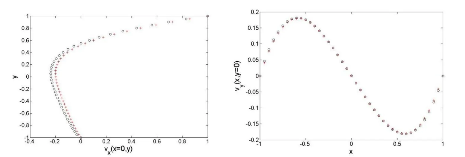
Figure 3:The pro files of vxat px=0along pyaxis and the pro files of vyat py=0 along pxaxis respectively(+:MFS,o:NMFS)using 196 boundary nodes in both methods and where for the MFS we chose RM=5d while for the NMFS we chose the radius Rin(42)equal d/4.

Figure 4:Comparison between the vxpro file at px=0 along the pyaxis computed with the MFS(+)with RM=5d and NMFS(o)when the number of nodes in MFS is kept fixed at 196 and the number of nodes N for NMFS is N=28,N=52,N=100 and R in(42)is equal to R=d/4,respectively(top to bottom).

Figure 5:Comparison between the vypro file at py=0 along the pxaxis computed with the MFS(+)with RM=5d and MMFS(o)when the number of nodes in MFS is kept fixed at 196 and the number of nodes N for MMFS is N=28,N=52,N=100 and R in(42)is equal to R=d/4,respectively(top to bottom).

Figure 6:The pro files of vxat px=0 along the pyaxis and the pro files of vyat py=0 along the pxaxis respectively,by using 100 boundary nodes in MFS and NMFS methods.Different values of R in(42)have been chosen when dealing with the NMFS method(+:MFS,o:NMFS with R=d/5,*=NMFS with R=d/4,-=NMFS with R=d/3).

In the third numerical experiment,we compare the numerical solutions obtained with MFS with respect to the one obtained with NMFS where the number of boundary nodes used for the latter increases(see Figs.4 and 5).

In Fig.6 we discussed the dependence of the NMFS solution upon the choices of the radius R in(46).We observe that the values of R in the interval(0,d/3]lead to a satisfactory reconstruction,however in agreement with Liu’s finding in[Liu(2010)]the choice R=d/4 is the optimal one.Such a choice is also consistent in solid mechanics[Liu and Šarler(2013)].

The condition numbers of the algebraic systems produced by NMFS are 2.14∗103,6.65∗103,1.5∗104for 100,196,292 number of nodes respectively.

Example 2:Circular computational domain with analytical solution

In the second example,the following analytical solution is considered[Young,Lin,Fan and Chiu(2009)]

where the circular computational domain Ω=A(0,0.5)is used and the Dirichlet boundary conditions are derived directly from the analytical solution.The aim of this example is to provide a validation by means of the comparison between the analytical solutions and the numerical solutions computed by the MFS and NMFS methods.

We used 600 equidistant boundary nodes picking the source points at a distanceRM=5d,where d is the smallest Euclidean distance between the two nodes when considering the MFS method,whereas,the numerical solutions computed by the NMFS have been obtained by keeping the number of boundary nodes fixed to 600 and by choosing R in(46)equal to d/4.In Fig.7,the pro files of the velocity alongpx=0 andpy=0 are presented respectively.

Fig.8 shows the relative error computed in the Euclidean norm of the differences between the analytical solution and the NMFS solution,measured along the pro file ofvyatpy=0 in 9 equidistant points on the interval(−0.5,0.5).The number of boundary nodes is from 225 to 2625.Moreover,we took into account the dependence of the error with respect to the choice of the parameterRin(46),where withNwe denote the number of the employed boundary nodes.

The condition number of the algebraic system produced by NMFS is 1.4∗105.

Figure 7:The pro files of vxat px=0 along pyaxis and the pro files of vyat py=0 along pxaxis respectively(+:MFS,o:NMFS,-:analytical solution).

Figure 8:The relationship between the relative errors and the number of boundary nodes for different R in(38)calculated by NMFS(+:R=d/3,*:R=d/4,o:R=d/5,).

Example 3:Flow in a channel

We consider a more practical example of flow in a channel which has been previously considered in[Fan,Li and Kuo(2011)].We make the following choice of the geometry Ω =(−2,2)× (−0.5,0.5)and the following choice for Dirichlet boundary data

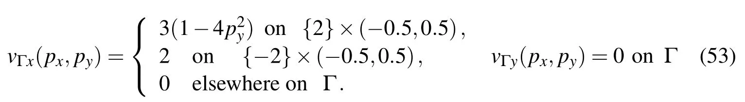
We assume no-slip boundary conditions on the upper and the bottom boundary,whereas a uniform in flow velocity is prescribed on the left boundary.Moreover,we consider a parabolic pro file of the out flow velocity on the right boundary.

First,we use the classical MFS to calculate the velocity field.We employ 960 equidistant boundary nodes as collocation points and we select the source points at a distance 5d from the physical boundary,where as usual d denotes the smallest distance between the two nodes.

In Fig.9 we compare the numerical solution presented in Figs.9 and 10,calculated by the MFS and the numerical solution computed by the NMFS where the radius R in(46)has been chosen equal to d/4.

Figure 9:Pro files of vxat px=0 along pyaxis and the pro files of vyat py=0 along pxaxis respectively(+:MFS,o:NMFS).

Figure10:The difference−of thepro files ofvxcomputed by the MFS and the NMF S method at px=0along pyaxis and the difference−of the profiles ofvy computed by the MFS and the NMFS method at py=0 along pxaxis respectively.

Let us observe that the NMFS solutions are essentially identical to the MFS one.Moreover,let us stress that by a visual comparison we can infer that our results are in good agreement with Trefftz method results obtained in[Fan,Li and Kuo(2011)]for the same example.

The condition number of the algebraic system produced by NMFS is 1.8∗105.

Example 4:Mixed Dirichlet-Fluid Traction boundary condition

We now solve the Stokes problem(1)and(2)in the rectangular domain Ω=(−2,2)×(−0.5,0)In this respect we consider the following analytical solution

We impose the following mixed Dirichlet-traction type boundary conditions

which are derived directly from the analytical solution.

Figure 11:Pro files of vxat px=0 along pyaxis and the pro files of vyat py=−0.25 along pxaxis respectively(+:MFS,o:NMFS).

We employed 1728 equidistant boundary nodes both for the MFS method and the NMFS method as well.We fixed the source points at distance RM=5d when dealing with the MFS method while we chose R in(46)equal to d/4 when treating the NMFS.In Fig.11,the pro files of the velocity alongpx=0 andpy=−0.25 are presented respectively.Let us observe that also for the mixed Dirichlet-traction boundary condition case,the analytical solution and the computed one are in good agreement.

The condition number of the algebraic system produced by NMFS is 1.04∗106.

5 Conclusions

In this paper,a combination of the NMFS and the Laplacian decomposition technique has been applied for the first time in order to solve a 2D Stokes flow problem with prescribed fluid velocity components along the boundary.By means of a suitable change of variables,we first reformulated the original Stokes system in terms of three Laplace equations satisfied by the new variables.The introduced harmonic functions are expanded as a linear combination of non-singular approximation functions.Moreover,we prescribe the continuity equation along the boundary which ensures that it is fulfilled in the domain as well.By a discretization argument we rephrased the problem at hand as a solution of a linear system of equation with unknown coefficients.We show the efficiency of the NMFS method by comparing the NMFS solutions with the MFS ones and,when available,with the analytical ones.The NMFS gives essentially the same results as the MFS,but has a great advantage that no artificial boundary is necessary.As a topic of future work we intend to extend the discussed method to 3D and to axisymmetry.Let us also mention that we believe that our technique can be successfully applied in study of inverse problems[Karageorghis,Lesnic and Marin(2011)],arising in the determination of unknown boundaries[Cabib,Fasino and Sincich(2011)]and unknown terms in boundary conditions[Sincich(2007);Sincich(2010)]by a single measurement.

Acknowledgement:This work was partially performed with in the Creative Core program(AHA-MOMENT)contract no.3330-13-500031,co-supported by RSMIZS and European Regional Development Fund Research;project J2-4093 Development and application of advanced experimental and numerical methods in karst processes,and program group P2-0379 Modelling and simulation of materials and processes,sponsored by Slovenian Grant Agency(ARRS).The authors wish to thank Prof.Daniel Lesnic for fruitful discussions on the topics of the paper.

Alves,C.J.S.;Silvestre,A.L.(2004):Density results using Stokeslet and a method of fundamental solutions for the Stokes equations.Engineering Analysis with Boundary Elements,vol.28,pp.1348-61.

Anderson,P.D.;Ternet,D.;Peters,G.W.M.;Meijer,H.E.H.(2006):Experimental/numerical analysis of chaotic advection in a three-dimensional cavity flow.International Polymer Processing,vol.21,pp.412-420.

Atluri,S.N.;Zhu,T.(1998):A new Meshless Local Petrov-Galerkin(MLPG)approach in computational mechanics.Computational Mechanics,vol.22,pp.117-127.

Avila,R.;Zhidong,H.;Atluri,S.N.(2011):A novel MLPG-Finite-Volume Mixed Method for Analyzing Stokesian Flows&Study of a new Vortex Mixing Flow.Computer Modeling in Engineering and Sciences,vol.71,pp.363-395.

Baf fico,L.;Grandmont,C.;Maury,B.(2010):Multiscale modeling of the respiratory tract.Mathematical Models&Methods in Applied Sciences,vol 20,pp.59-93.

Barrero-Gil,A.(2012):The method of fundamental solutions without fictitious boundary for solving Stokes problems.Computers&Fluids,vol.62,pp.86-90.

Barrero-Gil,A.(2013):The method of fundamental solutions without fictitious boundary for axisymmetric Stokes problems.Engineering Analysis with Boundary Elements,vol.37,pp.393-400.

Cabib,E.;Fasino,D.;Sincich,E.(2011):Linearization of a free boundary problem in corrosion detection.Journal of Mathematical Analysis and Applications,vol.387,pp.700-709.

Cao,H.;Pereverzev,S.;Sincich,E.(2014):Discretized Tikhonov regularization for Robin boundaries localization.Applied Mathematics and Computation,to appear.

Chantasiriwan,S.;Johansson,B.T.;Lesnic,D.(2009):The method of fundamental solutions for free surface Stefan problems.Engineering Analysis with Boundary Elements,vol.33,pp.529-39.

Chen,C.S.;Karageorghis,A.;Smyrlis,Y.S.(2008):The Method of Fundamental Solutions-A Meshless Method.Dynamic Publishers,Atlanta.

Cortez,R.(2001):The method of regularized Stokeslets.SIAM J.Sci.Comput.,vol.23,pp.1204-1225.

Cortez,R.;Fauci,L.;Medovikov,A.(2005)The method of regularized Stokeslets in three dimensions:Analysis,validation and application to helical swimming.Physics of Fluids,vol.17:doi:10.1063/1.1830486.

Curteanu,A.E.;Elliot,L.;Ingham,D.B.;Lesnic,D.(2007):Laplacian decomposition and the boundary element method for solving Stokes problems.Engineering Analysis with Boundary Elements,vol.31,pp.501-513.

Dong,L.;Alotaibi,A.;Mohiuddine,S.A.;Atluti,S.N.;Yusa,Y.;Yoshimura,S.(2014)Computational Methods in Engineering:A Variety of Primal&Mixed Methods,with Global&Local Interpolations,for Well-Posed or Ill-Posed Bcs.Computer Modeling in engineering&Sciences,vol.99,pp 1-85.

Fan,C.M.;Li,H.H.;Kuo,C.L.(2011):The modified collocation Trefftz method and Laplacian decomposition for solving two-dimensional Stokes problems.Journal of Marine Sciences and Technology,vol.19,pp.522-30

Gaspar,C.(2009):Several meshless solution techniques for the Stokes flow equations.In:Progress in Meshless Methods,Series:Computational Methods in Applied Sciences(ed.Ferreira AJM,Kansa EJ,Fasshauer GE,Leitao VMA),vol.11,pp 141-158.

Hwang,W.R.;Anderson,P.D.;Hulsen,M.A.(2005):Chaotic advection in a cavity flow with rigid particles.Physics of fluids,vol.17,043602.

Jana,S.C.;Metcalfe,G.;Otino,J.M.(1994):Experimental and computational studies of mixing in complex Stokes flows:the vortex mixing flow and multicellular cavity flows.J.Fluid Mechanics,vol.269,pp.199-246

Kang,T.G.;Hulsen,M.A.;Anderson,P.D.;den Toonder,J.M.;Meijer,H.E.H.(2007):Chaotic advection using passive and externally actuated particles in a serpentine channel flow.Chemical Engineering Science,vol.62,pp.6677-6686.

Karageorghis,A.;Lesnic,D.;Marin,L.(2011):A survey of applications of the MFS to inverse problems.Inverse Problems in Science and Engineering,vol.19,pp.09-36.

Kim,S.(2013):An improved boundary distributed source method for two dimensional Laplace equations.Engineering Analysis with Boundary Elements,vol.37,pp.997-1003.

Liu,Q.G.;Šarler,B.(2013):Non-Singular method of fundamental solutions for two-dimensional isotropic elasticity problems.CMES:Computer Modeling in Engineering and Sciences,vol.91,pp.235-66.

Liu,Q.G.;Šarler,B.(2014):Non-Singular method of fundamental solutions for anisotropic elasticity.Engineering Analysis with Boundary Elements,vol.45,pp.68-78.

Liu,Y.L.(2010):A new boundary meshfree method with distributed sources.Engineering Analysis with Boundary Elements,vol.34,pp.914-9.

Mramor,K.;Vertnik,R.;Šarler,B.(2013):Low and intermediate Re solution of lid driven cavity problem by local radial basis function collocation method.Computers,Materials&Continua,vol.36,pp.1-21.

Perne,M.;Šarler,B.;Gabrovšek,F.(2012):Calculating transport of water from a conduit to the porous matrix by boundary distributed source method.Engineering Analysis with Boundary Elements,vol.36,pp.1649-59.

Quarteroni,A.;Veneziani,A.(2003):Analysis of a geometrical multiscale model based on the coupling of ODE’s and PDE’s for blood flow simulations.Multiscale Modelling&Simulation,vol.1,pp.173-95.

Šarler,B.(2006):Solution of two-dimensional bubble shape in potential flow by the method of fundamental solutions.Engineering Analysis with Boundary Elements,vol.30,pp.227-35.

Šarler,B.(2009):Solution of potential flow problems by the modified method of fundamental solutions:Formulations with the single layer and the double layer fundamental solution.Engineering Analysis with Boundary Elements,vol.33,pp.1374-82.

Smith,D.J.(2009):A boundary element regularized Stokeslet method applied to cilia-and flagella–driven flow.Proc.R.Soc.A,vol. 465 doi:10/1098/rspa.2009.0295.

Sincich,E.(2007):Lipschitz stability for the inverse Robin problem.Inverse Problems,vol.23,pp.1311-26.

Sincich,E.(2010):Stability for the determination of unknown boundary and impedance with Robin boundary condition.SIAM Journal on Mathematical Analysis,vol.42,pp.2922-43.

Vignon-Clementel,I.E.;Figueroa,C.A.;Jansen,K.E.;Taylor,C.A.(2006):Out flow boundary conditions for the three-dimensional finite element modeling of blood flow and pressure in arteries.Computer Methods in Applied Mechanics and Engineering,vol.195,pp.3776-96

Wang,J.;Feng,L.;Otino,L.M.;Lueptow,R.(2009):Inertial effects on chaotic advection and mixing in a 2D cavity flow.Ind.Eng.Chem.Res.,vol.48,pp.2436-2442.

Young,D.L.;Jane,S.J.;Fan,C.M.;Murgesan,K.;Tsai,C.C.(2006):The method of fundamental solutions for 2D and 3D Stokes problems.Journal of Computational Physics,vol.211,pp.1-8.

Young,D.L.;Lin,Y.C.;Fan,C.M.;Chiu,C.C.(2009):The method of fundamental solutions for solving incompressible Navier-Stokes problems.Engineering Analysis with Boundary Elements,vol.33,pp.1031-1044.

Young,D.L.;Chen,K.H.;Lee,C.W.(2005):Novel meshless method for solving the potential problems with arbitrary domain.Journal of Computational Physics,vol.209,pp.290-322.