A New Approach to a Fuzzy Time-Optimal Control Problem

¸S.Emrah Amrahov,N.A.Gasilovand A.G.Fatullayev

1 Introduction

Many researchers have investigated optimal control problems with uncertainties.Gabasov,Kirillova,and Poyasok(2010a)have considered optimal preposterous observation and optimal control problems for dynamic systems under uncertainty with use of a priori and current information about the controlled object behavior and uncertainty.For an optimal control problem under uncertainty,Gabasov,Kirillova,and Poyasok(2009)have investigated the positional solutions,which are based on the results of inexact measurements of input and output signals of controlled object.In another study,Gabasov,Kirillova,and Poyasok(2010b)have studied a problem of optimal control of a linear dynamical system under set-membership uncertainty.Optimal control problem with uncertainty has firstly been formulated as a fuzzy optimal control problem by Filev and Angelov(1992).They have solved the problem on the basis of fuzzy mathematical programming and transformed the fuzzy problem to the multicriteria optimal control problem.

Sakawa et al.(1996)have proposed a fuzzy satisficing method for multiobjective linear optimal control problems.To solve these problems,they have discretized the time and replaced the system of differential equations by system of difference equations.Moon,VanLandingham,and Beliveau(1996)have developed a linear time varying state equation for hoisting and lowering operations of a crane system model.Wang(1998)have developed an optimal fuzzy controller for linear systems with quadratic cost function via Pontryagin’s Maximum Principle(PMP)[Pontryagin et al.(1986)].A fuzzy approach has been used by Kulczycki(2000)in the design of sub-time-optimal feedback controllers.

Fuzzy time-optimal control problems have been investigated in different forms by Plotnikov(2000);and Molchanyuk and Plotnikov(2009).Plotnikov(2000)has proved necessary maximin and maximax conditions for a control problem,when the behavior of the object is described by a controllable differential inclusion with multivalued performance criterion.Molchanyuk and Plotnikov(2009)have study the problem of high-speed operation for linear control systems with fuzzy right hand sides.For this problem,they have introduced the notion of optimal solution and established necessary and sufficient conditions of optimality in the form of the PMP.

A new fuzzy control system has been developed by Liu(2008)as an alternative approach to Mamdani(1974)and Takagi and Sugeno(1985)systems.Unlike the Mamdani and Takagi-Sugeno systems,the Liu fuzzy control system is not deterministic.Based on the concept of fuzzy Liu process,Zhao and Zhu(2010)have investigated a fuzzy optimal control model with a quadratic objective functional for a linear fuzzy control system.Likewise,based on Liu process a linear quadratic model have been proposed and the corresponding fuzzy optimal control problem have been solved by Qin,Bai,and Ralescu(2011).They have applied the approach to model production planning problems.

Nagi et al.(2011)have investigated fuzzy time-optimal control problem for second order nonlinear systems.A synthesis problem for fuzzy systems have been considered by Aliev,Niftiyev,and Zeynalov(2011).

In most of the application problems,the behavior of the object is determined by physics laws and is crisp.If the initial and final values are obtained from measurement,these values can be uncertain and often it is more adequate to model them by fuzzy numbers.Thus,optimal control problems arise with crisp dynamics but with fuzzy boundary values.In this paper,we consider such a problem.Namely,we consider a time-optimal control problem with crisp dynamics and with fuzzy start and target states.We interpret the optimal time as a fuzzy variable and propose a numerical method to calculate it.We demonstrate our method on a problem of fuzzy control of mathematical pendulum[Blagodatskikh(2001)].This problem is still an actual problem even in crisp case[Paoletti and Genesio(2011)],though it is investigated for a sufficiently long time.

The present paper consists of 6 sections including the Introduction.In Section 2,we give preliminaries on fuzzy sets and describe the classical time-optimal control problem.In Section 3,we define the fuzzy time-optimal control problem.In Section 4,we propose a method for calculation of fuzzy optimal time.In Section 5,we show the proposed approach by an example.Finally,we give concluding remarks in Section 6.

2 Preliminaries

2.1 Fuzzy sets

The notion of fuzzy set is an extension of the classical notion of set.In classical set theory,an element either belongs or does not belong to the given set.By contrast,in fuzzy set theory,an element has a degree of membership,which is a real number from[0,1],in the given fuzzy set.In fuzzy set theory,classical sets are usually called crisp sets.

For eachx∈U,is called the membership degree ofxin

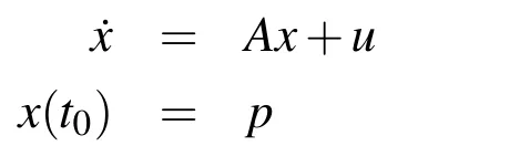
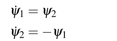
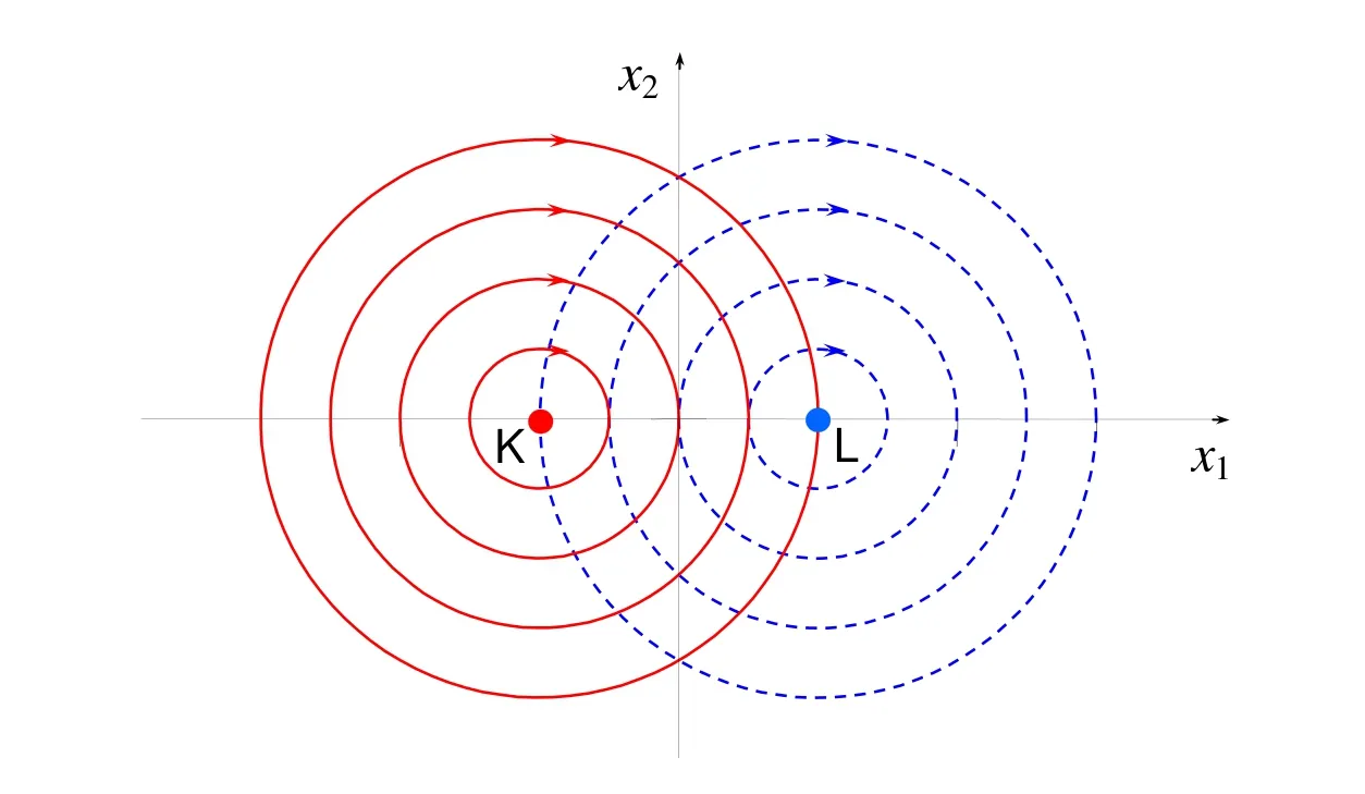
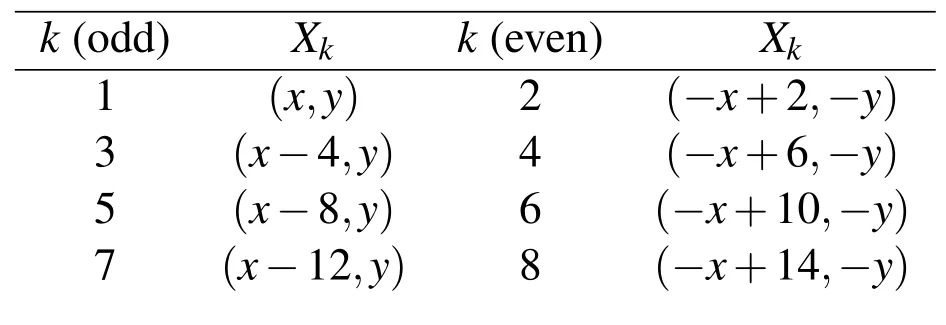
LetU=R(whereRis the set of real numbers).Let alsoa,candbbe real numbers such thata

is called a triangular fuzzy number and is denoted as

Fuzzy sets can be represented also via their α-cuts.

For each α ∈(0,1],the crisp setis called the α-cut ofFor α=0 we put

It is easy to see that if α increases,Aαcan only be narrower.Therefore,in the coordinate space,the α-cuts of a fuzzy set are bodies nested within one another.

2)is a bounded nonincreasing left-continuous function on(0,1]and right-continuous at α=0

Triangular fuzzy numbers are a particular case of fuzzy numbers in parametric form.For a triangular fuzzy numberwe haveand

2.2 Classical linear time-optimal control problem

Let the behavior of a controlled object be definite and described by the following linear system of differential equations:

Herexisn-dimensional vector-function that describes the phase state of the object,Ais ann×nmatrix,uisn-dimensional control vector-function.

LetU⊆Rnbe a nonempty compact set.If measurable functionu,defined on the intervalI=[t0,t1],satisfies the conditionu(t)∈Ufor eacht∈I,thenuis called an admissible control.It is known that for any admissible functionuand for any initial statepthe initial value problem

has a unique solution[Blagodatskikh(2001)].This solutionxdescribes how the phase state changes with time under the inf l uence of admissible controlu.

Assume that the start timet0and the start statepare given.If we want to transfer the object to a given stateqin the shortest time by choosing an appropriate admissible controlu,we have the following Classical time-optimal control problem of 1-st type:

Subject to

Note,that the finish timet1is not known beforehand and is determined as a result of solving the problem.Summarizing,1-st type classical time-optimal problem(2)-(5)is a problem of finding an admissible controlu,which transfers the object from the initial phase statepto the final phase stateqin the shortest time.

Now,let nonempty compact setsM0andM1fromRn,an intervalI=[t0,t1],and an admissible functionuon this interval be given.If the system(1)has a solutionx(t)such thatx(t0)∈M0andx(t1)∈M1,then it is said that the control functionutransfers the object from the initial phase setM0to the final phase setM1on the interval[t0,t1].If we want to transfer the object from the setM0to the setM1in the shortest time,we have the following Classical time-optimal control problem of 2-nd type:

Subject to

whereM0andM1are given start and target sets.The solutionuof the problem(6)-(9)is called optimal control.The solutionxof the system(7)-(9),corresponding to the optimal controlu,is called optimal trajectory.Ifu(t)is an optimal control andx(t)is a corresponding optimal trajectory,then(u(t),x(t))is called to be an optimal pair.

We note that the classical problem of 2-nd type can also be reformulated as follows:

2-nd type classical time-optimal problem(6)-(9)(or(10)-(13))is well studied[Pontryagin et al.(1986);Blagodatskikh(2001)].Below we give necessary conditions of optimality for this problem[Pontryagin et al.(1986);Blagodatskikh(2001)].

Definition 1.(Maximum principle).Let u be an admissible control defined on an interval[t0,t1]and let x be a solution of the system(7)-(9).We say that the pair(u(t),x(t))satisfies maximum principle on the interval[t0,t1]if the conjugate system

has such a nontrivial solution ψ =(ψ1,ψ2,...,ψn)that the following conditions hold:

1)maximum condition:hu(t),ψ(t)i=c(U,ψ(t))for almost any t∈ [t0,t1];

2)transversality condition on M0:hx(t0),ψ(t0)i=c(M0,ψ(t0));

3)transversality condition on M1:hx(t1),−ψ(t1)i=c(M1,−ψ(t1)).

HereA∗is the conjugate transpose matrix ofA(Note thatA∗=ATifAis a real matrix);hu,ψi=u1ψ1+u2ψ2+...+unψndenotes the inner product of vectorsuand ψ fromRnanddenotes the support function of the compact setSfromRn.

Theorem 1.[Blagodatskikh(2001)](Necessary conditions of optimality for the time-optimal control problem).Let M0and M1be nonempty convex compact sets.Also let the function u defined on[t0,t1]be an optimal control for the problem(6)-(9)and x be a corresponding optimal trajectory.Then the pair(u(t),x(t))satisfies maximum principle on the interval[t0,t1].

Remark 1:SinceM0andM1are nonempty compact sets and support functionc(·,ψ)is a linear function,the initial and final values of the optimal solutionx(t)of the problem(6)-(9)are achieved on boundaries of the setsM0andM1by Theorem 1.

3 Fuzzy linear time-optimal control problem

In most application problems,the behavior of the object is determined by laws of physics.Because of this the equations modeling the object’s behavior are crisp in nature.However,the initial and final states of the object may contain uncertainty.Depending on the nature of uncertainty,control problem can be modeled by different methods such as stochastic analysis,interval analysis,and fuzzy logic methods.For example,let the initial state be measured as a pointp=(a,b).Obviously,the certainty of this value depends on accuracy of the measuring device.If the measurement error is ε,then the initial state is a point from a square centered at(a,b)and with side length 2ε.If all points in this square are equivalent to each other as a candidate to the true value,then the problem can be modeled by interval analysis method.But often it is natural to expect that these points are not equivalent.For instance,degree of belief to the point(a,b)is more compared to any other point(x,y)from the square.And the degree of belief to(x,y)decreases as its distance from(a,b)increases.In this case,where the initial state is"close"to the measured value(a,b),it will be more appropriate to model the problem by means of fuzzy logic.In this paper,we consider such kind of model.For simplicity,we represent the"close"point’s coordinates(xandy)by fuzzy triangular numbers.

If the start and target values in classical problem of 1-st type are fuzzy,we obtain the following Fuzzy time-optimal control problem:

Subject to

In Fig.1 we give a schematic representation to problem(14)-(17)for the case of 2-dimensional phase space(i.e.x∈R2)

The problem shown in Fig.1 can be interpreted as follows:We want to transfer the object from start point to final point in the shortest time,where start point is"close"to(−5,3)and final point is"close"to(0,0).

Depending on definition of derivative of fuzzy function or definition of solution of system of differential equations,the problem(14)-(17)can be interpreted by different ways.For the present time,there are many difficulties with solving differential equations when fuzzy derivatives(such as Hukuhara,or generalized Hukuhara derivatives[Kaleva(1987);Bede and Gal(2005)])are used.Therefore,today it seems to be unproductive to apply fuzzy derivative for solving fuzzy optimal control problem.

We will interpret the problem(14)-(17)as a set of 1-st type classical problems(2)-(5).Each problem is obtained by taking the initial valuepfromand the final valueqfrom

Figure 1:Schematic representation for the problem(14)-(17)in phase space.The initial and final states and)are represented with fuzzy rectangles ABCD and EFGH,respectively.Dashed and dotted rectangles indicate α =0.3 and α =0.7-cuts.Dots represent the crisp values,the line connecting them depicts a crisp optimal trajectory.

De finition 2.Letanddenote the solutions of the problem(2)-(5).

Let also(wheredenotes the membership degreemembership degree α.

Set of allt1,pq,defined above,determines a fuzzy set.We will investigate how to calculateFunctionsandwhich indicate the left and right boundaries of α-cuts,determine the setfully.Thus,the problem of calculation of fuzzy optimal time is reduced to calculation of the functionsand

Lemma 2.(where α ∈ [0,1])is a solution of the following classical timeoptimal control problem of 2-nd type:

Proof.Ift1,pqis an optimal time with membership degreeµ≥α then,by the Definition 2,µeξ(p)≥α andµeζ(q)≥α,consequently,p∈ξαandq∈ζα(here ξαand ζαdenote α-cuts ofξeandζe,respectively).On the contrary,ifp∈ ξαandq∈ζαthen the corresponding solution has a membership degreeµ ≥α.is the shortest time among all solutions with membership degreeµ≥α.Therefore,can be obtained by solving the problem(6)-(9)with takingM0= ξαandM1= ζα,namely the problem(18)-(21).

Taking into account(10),it can be seen that

This formula can be used as alternative to(18)-(21)in numerical calculations.Note that,the valuemeans the shortest time between two points,one of them is from the set ξαand another is from ζα,in the best case.Similarly,means the shortest time in the worst case:

4 Numerical method to calculate the fuzzy shortest time

As it mentioned in Remark1,the initial and final states of the optimal trajectoryx(t)are achieved on boundaries of the sets ξαand ζα.Taking this fact into account we place equally spaced nodes on the boundaries of the regionsξαandζα.The shortest time among all possible start-destination node pairs(p,q)gives the approximate value ofaccording to the formula(22).Thus,to calculate the functionwe have to solvenα·n1·n2crisp problems of 1-st type(2)-(5).Heren1andn2denote the numbers of nodes approximating the boundaries of the regions ξαand ζα,respectively.

Similarly,to calculate the functionwe discretize the problem(23)and solve it numerically.

Remark 2:Considering of a fuzzy problem as a set of crisp problems becomes an effective tool in many cases,especially when other approaches fail.The main difficulty of this approach is that a set of crisp problems arises and new methods must be developed to combine their solutions in order to get a fuzzy solution.Gasilov,Amrahov,and Fatullayev(2011)applied the approach to the fuzzy initial value problem for linear system of differential equations;Gasilov,Amrahov,and Fatullayev(2013)and Gasilov et al.(2012)to the fuzzy boundary and initial value problems for high-order linear differential equation,respectively.

Note that the straightforward calculation of the functionby formula(22)requires to solvenα·n2·n2∼n5problems(2)-(5)(ifn×ngrids are used for initial and final sets).Lemma 2 and Remark 1 made it possible to reduce the number of calculations tonα·n·n∼n3.

5 Case study

In this section,we apply the proposed approach to a fuzzy time-optimal control problem.The problem is a fuzzified version of the crisp problem of damping of mathematical pendulum,presented in[Blagodatskikh(2001)].

Example 1.Solve the fuzzy time-optimal control problem(Note that below t0=0):

Hereare triangular fuzzy numbers.

Below the solution is given in 3 stages.

a)General notes and preliminary investigation.Initial and final state vectors,,form in the phase planeR2the fuzzy squares with sides of 1 and 0.5,and with centers at(−5,3)and(0,0),respectively(see,Fig.1).

It can be seen that ξα={(x1,x2)|α−6≤x1≤−4−α,α+2≤x2≤4−α}and ζα={(x1,x2)|0.5(α−1)≤x1≤0.5(1−α),0.5(α−1)≤x2≤0.5(1−α)}.The sets ξαand ζαalso are squares with the same centers aseξ andeζ,while with sides of 1−α and 0.5(1−α),respectively.

To solve the given fuzzy problem we need a solution method for the according crisp problem of 1-st type(2)-(5),which can be applied for arbitrary start statepand final stateq.Below,we develop such a method.

Support function ofUisc(U,ψ)=|ψ2|.Then,the maximum condition hu(t),ψ(t)i=c(U,ψ(t))impliesu2(t)ψ2(t)=|ψ2(t)|.Consequently,for optimal control we have:

The system’s matrix isA=.Sincethe conjugate system is

Let us find the solution of the conjugate system corresponding to an initial condition ψ(0)∈C,whereCis the unit circle.Initial points can be represented in the form of ψ(0)=(cosα,sinα)with α ∈ [0,2π).Then the solution of the conjugate system is ψ1(t)=cos(α −t),ψ2(t)=sin(α −t).The function ψ2(t)=sin(α −t)changes its sign for first time at τ≤π (τ=π if α =0;τ=α if 0<α ≤π;and τ=α−π if π < α <2π)and then after each π time period.Depending on α,the sign of the function ψ2(t)=sin(α −t)in the interval[0,τ]is either positive or negative.Thus,according to the maximum condition,the initial value of the optimal controlu2(t)is either 1 or−1.After τ≤π time units,it switches from 1 to−1 or vice versa.Then,it repeatedly changes its sign after each π time period.

Below we interpret the behavior of the object as a motion of the object in the phase planex1x2.

Solutions of dynamic system corresponding tou2(t)=1 are in the formx(t)=(1+ccos(ϕ −t),csin(ϕ −t)).In the phase planeR2these solutions constitute concentric circles with center atL(1,0)(Fig.2).The motion on these circles is clockwise with constant speed and whole turn takes 2π time units.

Similarly,solutions of dynamic system corresponding tou2(t)=−1 are in the formx(t)=(−1+ccos(ϕ−t),csin(ϕ−t)).InR2these solutions constitute circles with center atK(−1,0)(Fig.2).The motion on these circles is clockwise with constant speed and whole turn takes 2π time units.

Figure 2:An optimal trajectory can be realized by combining of clockwise motions on circles with centers K and L.

Note that angular speed is ω=1 for both motions mentioned above.So,the angle formed by the object during its motion and the passed time are equal in value.

Let us emphasize two facts which will be used in arguments below.1)In circular motion with ω =1 after π time period the object will be in the position which is opposite(central symmetric point)of the current position.2)The symmetric point of(a,b)is(−a−2,−b)with respect to center pointK.If center isL,then the symmetry of point(c,d)is(−c+2,−d).

b)Semi-analytical solution of 1-st type crisp problem.Now we investigate how is a motion of the object corresponding to an optimal control in the phase plane for a start pointSand a target pointT.Let us consider the case when the object starts with controlu=−1(The case with start controlu=1 can be investigated similarly).Letkdenote the number of control switches.We consider the casesk=0(motion without switch)andk≥1 separately.

In the casek=0,running from the start positionSand moving along a circle with centerKthe object reaches the target positionT.This case occurs,only if|KS|=|KT|(Here|AB|denotes the length of the segmentAB).The motion time ist1=θ=∠SKT(Here∠SKTdenotes the value of the angleSKT).

Now letk≥1.We differ the cases whenkis odd and whenkis even.

Figure 3:A sample of optimal trajectory with 3 switches.

Let us consider the case thatkis odd number and takek=3 for clarity.The object runs from the pointSalong a circle with centerKand after τ time period arrives a pointX1(x,y)(Fig.3).The pointsSandX1are on the same circle.Consequently:

At the pointX1the control switches for the first time and becomesu=1.Under this control,the object moves along a circle with centerL.After π time units it arrives a pointX2(−x+2,−y).Here the control switches for the second time and under new controlu= −1(moving on circle with centerK)after π time the object reaches a pointXk=X3(x−4,y).At the pointXkthe control switches for last time and becomesu=1.The object continues its motion on a circle with centerLup to the target pointT.For the aforementioned motion,the pointsXkandTmust be on the same circle with centerL,i.e.,

It can be seen from Table 1 that for an oddk(includingk=1)the last point of control switch is

Table 1:Point of k-th control switch for optimal motion

LetS=(px,py)andT=(qx,qy).To calculate unknown coordinatesxandywe use equations(24)and(25).Using(26),these equations can be rewritten in coordinates as follows:

Subtracting(28)from(27)we have:4k(x+1)−4k2=−.Then we can determinexandyas follows:

Ifxandyhave been determined we can calculate the passed time:

Let us find an evaluation fork.From(29)and(30)we have

Hence,we obtain the following evaluation

Then,we havekopt

The case whenk≥1 andkis even can be investigated by similar way.In this case the last point of the control switch is(see,Table 1):

The last control isu=−1 and,consequently,the object finishes its motion on a circle with centerK.Hence,.Except this value,the formulas forxandybecome the same as(29)and(30).The motion time is:

Above we have investigated the case when the start controluequals to−1.In the case whereuis 1 we have the following final formulas:

The above formulas,given for different situations,were obtained on the base of the necessary conditions for optimality.Therefore,every solution constructed on these formulas may not be optimal.However,the optimal solution is among all solutions,constructed for different start controls and for different values ofk.

Based on the above arguments and formulas a computer program is implemented to calculate the optimal control for a given pair of start pointSand target pointT.Firstly,by taking start controlu=−1,after takingu=1 and in both cases by changing the value ofkfromkmintokmaxa solution is constructed(if there is any).The solution with the shortest time is the optimal solution,transferring the object fromStoT.

Figure 4:The membership function of fuzzy optimal time

c)Results of the numerical calculations.The membership function of fuzzy optimal timeobtained from calculations,is depicted in Fig.4.Although the initial and final states are expressed by fuzzy triangular numbers,we can see thatis not triangular.The valuet1≈8.78 with membership degree 1 corresponds to the solution of the crisp problem(p=(−5,3)andq=(0,0).The corresponding optimal trajectory is shown in Fig.1.The least valuet1≈5.97 with membership degree 0 occurs whenp=(−4,2)andq=(−0.5,0.5).The largest valuet1≈11.76 with membership degree 0 corresponds to the pairp=(−6,4)andq=(0.5,0.5).We can note the following in regard to the obtained solution.The solution of according crisp problem is≈8.78.When the initial and final states are fuzzy it could be expected that the optimal time would be a fuzzy number with vertex atThe obtained solution determines the parameters of this fuzzy number:the size of the uncertainty(i.e.how wide is it),its shape(is it triangular or not,etc.).

6 Conclusion

In this paper,we investigated the time-optimal control problem with fuzzy initial and final states.We interpreted the problem as a set of crisp problems.This approach allows to transform a fuzzy problem to a set of crisp problems,that can be solved with known methods.The approach can be applied to the problems when the behavior of the object is described by the system of differential equations or by the higher-order differential equation.As it is known,the application of the Hukuhara or generalized derivatives to these problems is difficult because the number of cases have to be analyzed increases exponentially with order.

Based on the approach we proposed a numerical method to solve the fuzzy time optimal control problem.The complexity of the method isO(n3)for the2-dimensional phase space,ifn×ngrids are used for the initial and final sets.

We demonstrated the proposed method on a numerical example.To solve the arising crisp time-optimal control problem of 1-st type we developed a numerical algorithm.Also,we showed how to obtain the fuzzy solution from the solutions of the corresponding crisp problems.

Acknowledgement:This work is supported by Scientific and Technological Re

search Council of Turkey(TUBITAK)under the project ID 114E269.

Aliev,F.A.;Niftiyev,A.A.;Zeynalov,C.I.(2011):Optimal synthesis problem for the fuzzy systems,Optim.Control Appl.Meth.,vol.32,pp.660–667.

Bede,B.;Gal,S.G.(2005):Generalizations of the differentiability of fuzzy number valued functions with applications to fuzzy differential equation,Fuzzy Sets and Systems,vol.151,pp.581–599.

Blagodatskikh,V.I.(2001):Introduction to Optimal Control[in Russian],Vysshaya Shkola,Moscow.

Filev,D.;Angelov,P.(1992):Fuzzy optimal control,Fuzzy Sets and Systems,vol.47,issue 2,pp.151–156.

Gabasov,R.;Kirillova,F.M.;Poyasok,E.I.(2009):Robust optimal control on imperfect measurements of dynamic systems states,Appl.Comput.Math.,vol.8,issue 1,pp.54–69.

Gabasov,R.;Kirillova,F.M.;Poyasok,E.I.(2010):Optimal real-time control of nondeterministic models on imperfect measurements of input and output signals,TWMS J.Pure Appl.Math.,vol.1,issue 1,pp.24–40.

Gabasov,R.;Kirillova,F.M.;Poyasok,E.I.(2010):Optimal control of linear systems under uncertainty,Proceedings of the Steklov Institute of Mathematics,vol.268,supplement 1,pp.95–111.DOI:10.1134/S0081543810050081

Gasilov,N.A.;Amrahov,¸S.E.;Fatullayev,A.G.(2011):A geometric approach to solve fuzzy linear systems of differential equations,Appl.Math.Inf.Sci.,vol.5,pp.484–495.

Gasilov,N.;Amrahov,¸S.E.;Fatullayev,A.G.(2013):Solution of linear differential equations with fuzzy boundary values,Fuzzy Sets and Systems.http://dx.doi.org/10.1016/j.fss.2013.08.008

Gasilov,N.A.;Hashimoglu,I.F.;Amrahov,¸S.E.;Fatullayev,A.G.(2012):A new approach to non-homogeneous fuzzy initial value problem,CMES:Computer Modeling in Engineering&Sciences,vol.85,issue 4,pp.367–378.

Kaleva,O.(1987):Fuzzy differential equations,Fuzzy Sets and Systems,vol.24,pp.301–317.

Kulczycki,P.(2000):Fuzzy controller for mechanical systems,IEEE Transactions on Fuzzy Systems,vol.8,issue 5,pp.645–652.

Liu,B.(2008):Fuzzy process,hybrid process and uncertain process,Journal of Uncertain Systems,vol.2,issue 1,pp.3–16.

Mamdani,E.H.(1974):Applications of fuzzy algorithms for control of simple dynamic plant,Proceedings of the Institution of Electrical Engineers“Control&Science”,vol.121,issue 12,pp.1585–1588.

Molchanyuk,I.V.;Plotnikov,A.V.(2009):Necessary and suf ficient conditions of optimality in the problems of control with fuzzy parameters,Ukrainian Mathematical Journal,vol.61,issue 3,pp.457–466.

Moon,M.S.;VanLandingham,H.F.;Beliveau,Y.J.(1996):Fuzzy time optimal control of crane load,in:Proceedings of the 35th Conference on Decision and Control,Kobe,Japan,December 1996,pp.1127–1132.

Nagi,F.;Ahmed,S.K.;Zularnain,A.T.;Nagi,J.(2011):Fuzzy time-optimal controller(FTOC)for second order nonlinear systems,ISA Transactions,vol.50,pp.364–375.

Paoletti,P.;Genesio,R.(2011):Rate limited time optimal control of a planar pendulum,Systems&Control Letters,vol.60,pp.264–270.

Plotnikov,A.V.(2000):Necessary optimality conditions for a nonlinear problem of control of trajectory bundles,Cybernetics and Systems Analysis,vol.36,issue 5,pp.730–733.

Pontryagin,L.S.;Boltyanskii,V.G.;Gamkrelidze,R.V.;Mishchenko,E.F.(1986):The Mathematical Theory of Optimal Processes(ISBN 2-88124-134-4),Gordon and Breach Science Publishers,New York.

Qin,Z.;Bai,M.;Ralescu,D.(2011):A fuzzy control system with application to production planning problems,Information Sciences,vol.181,pp.1018–1027.

Sakawa,M.;Inuiguchi,M.;Kato,K.;Ikeda,T.(1996):A fuzzy satis ficing method for multiobjective linear optimal control problems,Fuzzy Sets and Systems,vol.78,pp.223–229.

Takagi,T.;Sugeno,M.(1985):Fuzzy identification of systems and its applications to modelling and control,IEEE Transactions on Systems,Man and Cybernetics,vol.15,issue 1,pp.116–132.

Wang,L.-X.(1998):Stable and optimal fuzzy control of linear systems.IEEE Trans.Fuzzy Sys.,vol.6,issue 1,pp.137–143.

Zhao,Y.;Zhu,Y.(2010):Fuzzy optimal control of linear quadratic models,Computers and Mathematics with Applications,vol.60,pp.67–73.