Block methods for linear Hamiltonian systems

TIAN Hongjiong, CHEN Bailin

(College of Mathematics and Sciences,Shanghai Normal University,Shanghai 200234,China)

1 Introduction

The time integration of ordinary differential equations (ODEs) is a classical topic of numerical mathematics.In the traditional approach,one-step methods like Runge-Kutta methods and multistep methods like Adams methods and BDF are constructed with a high order of convergence and favourable stability properties (see,e.g.,Butcher[1],Hairer,Nørsett and Wanner[2],Hairer and Wanner[3]and Lambert[4]).One- and multi-block methods,and boundary value methods can be regarded as a set of linear multistep methods simultaneously applied to ODEs and then combined to yield an approximation with high accuracy,better stability and efficiency in parallel computing (see,e.g.,Axelsson and Verwer[5],Bond and Cash[6],Brugnano and Trigiante[7-11],Chartier[12],Chu and Hamilton[13],Lu[14],Shampine and Watts[15],Sommeijer,Couzy and van der Houwen[16],Tian,Shan and Kuang[17],Tian,Yu and Jin[18],Watanabe[19],Watts and Shampine[20],and Zhou[21]).

Many technical or physical models are described by Hamiltonian systems.The study of Hamiltonian systems has a very long history,while their numerical solution is a more recent field of investigation,which has led to the definition of symplectic or canonical integrators.The known symplectic integrators are essentially Runge-Kutta schemes,while there are no high order symplectic integrators in the class of linear multistep methods (see,e.g.,Eirola and Sanz-Serna[22],Feng and Qin[23],Hairer,Lubich and Wanner[24],Sanz-Serna and Calvo[25],Tang[26]).Recently,several classes of symplectic boundary value methods have been proposed for linear Hamiltonian systems (see,Brugnano[27],Brugnano and Trigiante[7]).For the conservation of energy of polynomial Hamiltonian systems of boundary value methods by means of discrete line integral,we refer to Brugnano,Iavernaro and Trigiante[28],Iavernaro and Pace[29].

In this paper,we shall restrict our analysis to the following linear Hamiltonian problem

y′(t)=Ly(t),t∈[t0,T],

y(t0)=y0,

(1)

wherey(t)∈2m,Imdenotes the identity matrix of orderm,L=J2mS,S=ST∈2m,and

⊗Im.

The main features of this linear Hamiltonian problem are

(a)Q(hL)=ehJ2mSis a symplectic matrix forh>0,that is,Q(hL)TJ2mQ(hL)=J2m, and

(b) for every matrixCsuch thatLTC+CL=0,the quadratic formV(t;C)=y(t)TCy(t) is a constant of motion.

In particular,forC=S,one obtains the Hamiltonian function of the problem.One wishes to construct numerical methods such that the properties (a) and (b) are preserved.

In Sections 2,we shall briefly recall the block methods for ordinay differential equations.In Section 3,we discuss the application of the block methods to linear Hamiltonian problems.In Section 4,we show that thek-dimensional block method which is convergent of order at leastk+1 is symplectic and preserves the quadratic form at the last point of the block fork=1,2,…,8. Finally,in Section 5,we present some numerical results to illustrate the performance of the block methods.

2 Block Methods

We first briefly recall the block method for the initial value problem

y′(t)=f(t,y(t)),t∈[t0,T],

y(t0)=y0,

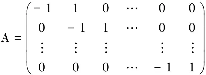
wherey0,yandfares-vectors.Leth>0 be a constant step size,kbe a given positive integer,l=nkandn=0,1,2,…,andtl=t0+lh.Thek-dimensional implicit block method is in the form

A⊗IsYn=a⊗Isyl+hB⊗IsF(Yn)+hb⊗Isfl,

(2)

whereYn=[ynk+1T,…,ynk+kT]T∈sk,F(Yn)=[fnk+1T,…,fnk+kT]T∈sk,fl+i=f(tl+i,yl+i),yl+iapproximatesy(tl+i),i=0,1,…,k,A∈k×kis assumed to be invertible,B∈k×kanda,b∈k.When the coefficient matricesA,Band the vectorsa,bare determined,one obtains a discrete set ofknew solution values fromyl.SinceAis assumed to be invertible,the block method (2) is equivalent to

(3)

We now give the first result on zero-stability of the block method.

ProofIt follows from (2) that

Yn+1=[0,0,…,A-1a]⊗IsYn+h(A-1B)⊗IsF(Yn+1)+h[0,0,…,A-1b]⊗IsF(Yn).

(4)

Note that the eigenvalues of the matrix [0,0,…,A-1a] consists of zeros with multiplicityk-1 and the last component ofA-1a. This completes the proof.

In order to study the consistency and convergence of the block method,we define the local truncation error of (3) as

(5)

where

Zn=[y(tnk+1),y(tnk+2),…,y(tnk+k)]T∈sk.

LetK1i=[1i,2i,…,ki]T∈k,i=0,1,2,…,ande=[1,1,…,1]T∈k.Using Taylor expansion ofy(t) attl,we can obtain the expression of the local truncation error

L[Zn,h]=d0⊗Isy(tl)+hd1⊗Isy(1)(tl)+…+hpdp⊗Isy(p)(tl)+…,

where

(6)

The block method is consistent of at leastpth-order if

dj=0,j=0,1,…,p.

Theorem2.2For any integerk,there exists a uniquek-dimensional block method (3) which is convergent of order at leastk+1.

The following result has been proven by Watts and Shampine[20].

Theorem2.3[20]Consider thek-dimensional block method obtained in Theorem 2.2.Fork=1,2,…,8,the corresponding block method isA-stable and convergent of orderk+1 forkodd and of orderr+2 forkeven.Forr=9,10,the method is not A-stable.

3 Application of Block Methods to Linear Hamiltonian Systems

Introducing

Yn=(ynkT,ynk+1T,…,ynk+kT)T,F(Yn)=(fnkT,fnk+1T,…,fnk+kT)T,

we may rewrite the block method (2) in a compact form

A ⊗I2mYn=hB ⊗I2mF(Yn),

(7)

where

(8)

and

(9)

Application of the block method (7) to problem (1) yields

A⊗I2mYn=hB ⊗J2mSYn.

(10)

In other words,the vector Ynsatisfies the equation

MY:=(A ⊗I2m-hB ⊗J2mS)Y=0.

(11)

The discrete solution is obtained by solving the linear system

(12)

In order to obtain the most appropriate block methods for problem (1),we shall follow the way proposed by Brugnano and Trigiante[7].By changing the independent variableτ=T-t,we observe that

(13)

which is still Hamiltonian.This implies that the same numerical method should provide the same discrete solution in the reverse order.Define

Zn=(Pk+1⊗I2m)Yn≡(ynk+k,…,yn+1,yn)T,

wherePk+1=[ek+1,ek,…,e1] is a permutation matrix,eiis theith vector of the canonical base ink+1.Suppose that

PkAPk+1=-A,PkBPk+1=B.

(14)

Then,multiplication of the left side of (11) byPk⊗I2mgives

(15)

Therefore,Zncan be obtained by direct application of the block method to (13).

The symmetry conditions in (14) will play an important role in the derivation of conservation laws for the discrete system.

We first give some preliminary results and symbols.LetQ0andQ1be the permutation matrices of dimensions (k+1)2andk2such that

(16)

Furthermore,we take the following partitioning

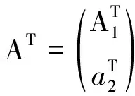
A=(A1,a2), B=(B1,b2),a2,b2∈k,

(17)

and define

(18)

For any givenφ∈(k+1)2satisfying

(Pk+1⊗Pk+1)φ=-φ,Q0φ=φ,

(19)

we consider the following linear system

(AT⊗BT+BT⊗AT)η=φ,

(20)

where the unknown vectorη∈k2.

Lemma3.1Suppose that (14) is satisfied and R defined in (18) is nonsingular.Then,for anyφsatisfying (19),there exists a unique solutionηof (20),which also satisfies the relations

(Pk⊗Pk)η=η,Q1η=η.

(21)

ProofThe proof of this lemma is similar to that given by Brugnano and Trigiante[7].According to the partitioning in (17),we have

(22)

It follows from the hypothesis,R is nonsingular,that the coefficient matrix of Equation (20) has full column rank.We shall prove later that the remaining equations are redundant,so that there exists a unique solution vectorηof (20).We first show (21) holds whenηis a solution of (20).In fact,from (14),one has that

(23)

Thusηis a solution of (20) iff (Pk⊗Pk)ηis also a solution.The first equality in (21) then follows from the fact that the coefficient matrix (22) has full column rank.Similarly,the second equality follows by the relation

φ=Q0φ=Q0(AT⊗BT+BT⊗AT)Q1Q1η=(BT⊗AT+AT⊗BT)Q1η.

(24)

(25)

where the last equality follows from (19).From (14),it follows that

Thus

(26)

which shows that the first and the last equations in (20) are equivalent.This completes the proof.

We have the following main result.

Theorem3.2Suppose that the hypotheses of Lemma 3.1 are satisfied,andCis a matrix such thatCL+LTC=0.Then,the solution of system (11) satisfies

(27)

for alli,j=0,1,…,k.

ProofThe proof is similar to that given by Brugnano and Trigiante[7]and is omitted.

The discrete conservation corresponding to the property (b) in Section 1 can now be easily shown.

Corollary3.3Suppose that the hypotheses of Lemma 3.1 are satisfied.Then the constants of motion of problem (1) are exactly preserved in the last point of each block.

ProofLetCbe any matrix such thatCL+LTC=0.Takingi=j=0 in (27),we obtain

This completes the proof.

RemarkWhenC=S, the conservation for the Hamiltonian function holds.Moreover,from (27) andj=i,one obtains that

that is,the approximations of the constants of motion are symmetric in each block.

In Section 1,it was remarked that for eachh,the mapQ(hL) is symplectic for the continuous flow,which is the property (a).A similar result holds for the discrete map associated with the method described by Equation (12).Introducing the block vector

(28)

we see that itsith block entry defines the mapynk+i=φiynk.Moreover,the block vectorΦsatisfies Equation (11).It follows from Theorem 3.2 withC=J2mthat

(29)

As a consequence,we obtain the discrete analog of the property (a).

Corollary3.4Suppose that the hypotheses of Lemma 3.1 are satisfied.Then the mapynk+k=φkynkis symplectic.

ProofNote thatφ0=I2m.Fori=j=0,(29) gives

This completes the proof.

4 Some Examples

We now present somek-dimensional block methods of order at leastk+1 such that the conditions in Theorem 3.2 hold.

Example1Fork=1,the symplectic block method is

(30)

and is equivalent to the trapezoidal rule

Example2Fork=2,we propose the block method with

whereα≠±1 is a parameter.It can be verified that it is zero-stable,di=0,i=0,1,2,3,P2AP3=-A,P2BP3=B,and R is invertible.It is also equivalent to

(31)

Example 3 Fork=3,we propose the block method with

and

whereα,β,γ,ζare parameters such thatα≠ -1 andγ+ζ-αζ-2βγ≠ 0.It can be verified that it is zero-stable,di=0,i=0,1,2,3,4,P3AP4=-A,P3BP4=B,and R is nonsingular.This block method is also equivalent to

(32)

Example 4 Fork=4,5,6,7,8,we propose the block methods with

and B as follows (table 1).

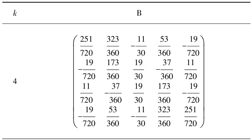
Table 1 Coefficients of block methods for 4≤k≤8

Table 1(continued)

It can be verified that each block method is zero-stable,di=0,i=0,1,…,k+1,PkAPk+1=-A,PkBPk+1=B,and R is nonsingular.These methods are equivalent to

Yn=eyl+hBF(Yn)+hbfl,

(33)

wheree=(1,1,…,1)T,Bandbare as follows (table 2).

Table 2 Coefficients of block methots 4≤k≤8

Table 2(continued)

According to the equivalence,we have the following main result.

Theorem 4.1 Consider thek-dimensional block method obtained in Theorem 2.2.Fork=1,2,…,8,the properties in Theorem 3.2 and Corollaries 3.3 and 3.4 hold for the corresponding block method.

5 Numerical Experiment

We illustrate the performance of the 4- and 8-dimensional block methods given in the previous section by integrating the system of harmonic oscillator

(34)

The Hamiltonian function of (34) isV(t)=9y1(t)2+y2(t)2.

Figure 1 Discrete values yr (left) and Vr (right) with

Figure 2 Discrete values yr (left) and Vr (right) with

Figure 3 Discrete values yr (left) and Vr (right) with

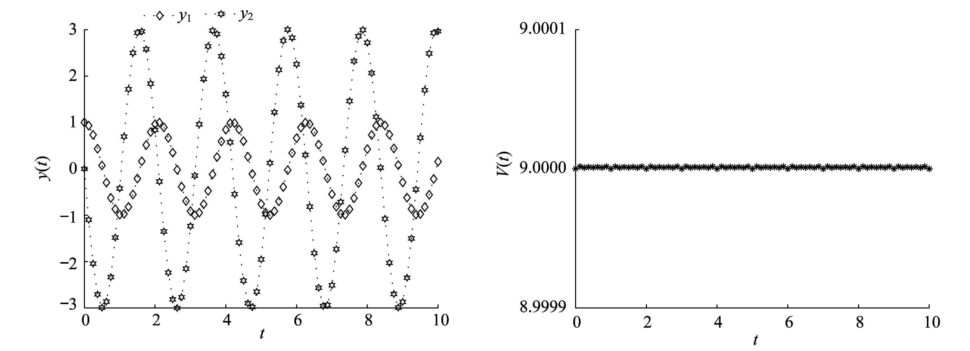
Figure 4 Discrete values yr (left) and Vr (right) with

:

[1] BUTCHER J C.Numerical Methods for Ordinary Differential Equations[M].New York:Wiley Chichester,2008.

[2] HAIRER E,NØRSETT S P,WANNER G.Solving Ordinary Differential Equations I:Nonstiff Problems[M].2nd Edition,Berlin:Springer-Verlag,1993.

[3] HAIRER E,WANNER G.Solving Ordinary Differential Equations II:Stiff and Differential-Algebraic Problems[M].2nd Edition,Berlin:Springer Verlag,1996.

[4] LAMBERT J D.Numerical Methods for Ordinary Differential Systems[M].NJ:John Wiley & Sons,Inc.,1991.

[5] AXELSSON A O H,Verwer J G.Boundary value techniques for initial value problem in ordinary differential equations[J].Math Comp,1985,45:153-171.

[6] BOND J,CASH J R.A block method for the numerical integration of stiff systems of ordinary differential equations[J].BIT,1979,19:429-447.

[7] BRUGNANO L,TRIGIANTE D.Block boundary value methods for linear Hamiltonian systems[J].Appl Math Comp ,1997,81:49-68.

[8] BRUGNANO L,TRIGIANTE D.High order multistep methods for boundary value problems[J].Appl Num Math,1995,18:79-96.

[9] BRUGNANO L,TRIGIANTE D.Convergence and stability of boundary value methods for ordinary differential equations[J].J Comp Appl Math,1996,66:97-109.

[10] BRUGNANO L,TRIGIANTE D.Boundary value metheds:the third way between linear multistep and Runge-Kutta methods[J].Comp Math Appl,1998,36:269-284.

[11] BRUGNANO L,TRIGIANTE D.Solving ODEs By Multistep Initial and Boundary Value Methods[M].Amsterdam:Gordon & Breach,1998.

[12] CHARTIER P.L-stable parallel one-block methods for ordinary differential equations[J].SIAM J Numer Anal,1994,31:552-571.

[13] CHU M,HAMILTON H.Parallel solution of ODEs by multi-block methods[J].SIAM J Sci Stat Comput,1987,8:342-353.

[14] LU L.The stability of the blockθ-methods[J].IMA J Numer Anal,1993,13:101-114.

[15] SHAMPINE L F,WATTS H A.Block implicit one-step methods[J].Math Comp,1969,23:731-740.

[16] SOMMEIJER B P,COUZY W,van der HOUSEN P J.A-stable parallel block methods for ordinary and integro-differential equations[J].Appl Numer Math,1999,81:451-459.

[17] TIAN H,SHAN K,KUANG J.Continuous blockθ-methods for ordinary and delay differential equations[J].SIAM J Sci Comp,2009,31:4266-4280.

[18] TIAN H,YU Q,JIN C.Continuous block implicit hybrid one-step methods for ordinary and delay differential equations[J].Appl Numer Math,2011,61:1289-1300.

[19] WATANABE D S.Block implicit one-step methods[J].Math Comput,1978,32:405-414.

[20] WATTS H A,SHAMPINE L F.A-stable implicit block one-step methods[J].BIT,1972,12:252-266.

[21] ZHOU B.A-stable andL-stable block implicit one-step methods[J].J Comp Math,1985,3:328-341.

[22] EIROLA T,SANZ-SERNA J M.Conservation of integrals and symplectic structure of differential equations by multistep methods[J].Numer Math,1992,61:281-290.

[23] FENG K,QIN M Z.Sympletic Geometric Algorithms for Hamiltonian Systems[M].Hangzhou:Zhejiang Science and Technology Press,2003.

[24] HAIRER E,LUBICH C,WANNER G.Geometric Numerical Integration:Structure-Preserving Algorithms for Ordinary Differential Equations[M],2nd Edition∥Springer Series in Computational Mathematics.Berlin:Springer-Verlag,2006.

[25] SANZ-SERNA J M,CALVO M P.Numerial Hamiltonian Problems[M].London:Chapman & Hall,1994.

[26] TANG Y F.The symplecticity of multi-step methods[J].Comput Math Appl,1993,25:83-90.

[27] BRUGNANO L.Essentially symplectic boundary value methods for linear Hamiltonian systems[J].J Comp Math,1997,15:233-252.

[28] BRUGNANO L,IAVENARO F,TRIGIANTE D.Hamiltonian Boundary Value Methods (Energy Preserving Discrete Line Integral Methods)[J].J Numer Anal Indu Appl Math,2010,5:17-37.

[29] IAVERNARO F,PACE B.Conservative block-boundary value methods for the solution of polynomial Hamiltonian systems[J].AIP Conf Proc,2008,1048:888-891.