The First Initial Boundary Value Problem for Parabolic Hessian Equations on Riemannian Manifolds

REN CHANG-YU

(School of Mathematics,Jilin University,Changchun,130012)

Communicated by Yin Jing-xue

The First Initial Boundary Value Problem for Parabolic Hessian Equations on Riemannian Manifolds

REN CHANG-YU

(School of Mathematics,Jilin University,Changchun,130012)

Communicated by Yin Jing-xue

For a class of elliptic Hessian operators,one type of corresponding parabolic Hessian equations is studied on Riemannian manifolds.The existence and uniqueness of the admissible solution to the first initial boundary value problem for the equations are shown.

Hessian operator,fully nonlinear,Riemannian manifold

1 Introduction

In this paper,we study the first initial boundary value problem for a class of fully nonlinear parabolic equations of Monge-Amp`ere type on Riemannian manifolds.Let Ω be a domain of a Riemannian manifold(Mn,g)with n≥2.We consider the following problem:

The problem(1.1)with Hessian operators constitute an important class of fully nonlinear equations.The study on Dirichlet problem of(1.1)containing Hessian operator initiated from[1].It is well known that the classic Monge-Amp`ere operator is one of Hessian operators. General elliptic Hessian equations have been studied by[2–6].In 1999,the existence anduniqueness of solution to the Dirichlet problem of elliptic equation which contains Hessian operator were established in[3].For the parabolic case,it seems that the discussion on the equations with Hessian operators initiated from[7].However,the operators are not of the common form.Ren[8]extended the result of[7],and Wang and Liu[9]studied another type of equations,i.e.,

In 1996,the Dirichlet problem for elliptic Monge-Amp`ere equation on Riemannian manifolds was investigated in[10].

Ren and Wang[11]have discussed a type of parabolic Monge-Amp`ere equations which was introduced by Krylov[12].In this paper,we generalize our former work and establish the existence and uniqueness of solution to the first initial boundary value problem for parabolic equation which contains Hessian operator.

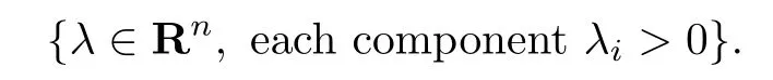
Throughout this paper,let f(λ)be a smooth function defined in an open convex cone Γ⊂Rnwith vertex at the origin and containing the positive cone

It satisfies that for any i,

and

Assume that Γ and f are invariant under interchange of any two λi,namely,they are symmetric in λi.It follows that Γ⊂{∑λi＞0}.For every C＞0 and every compact set K in Γ there is a number R=R(C,K)such that

In addition,as in[3],assume that f satisfies

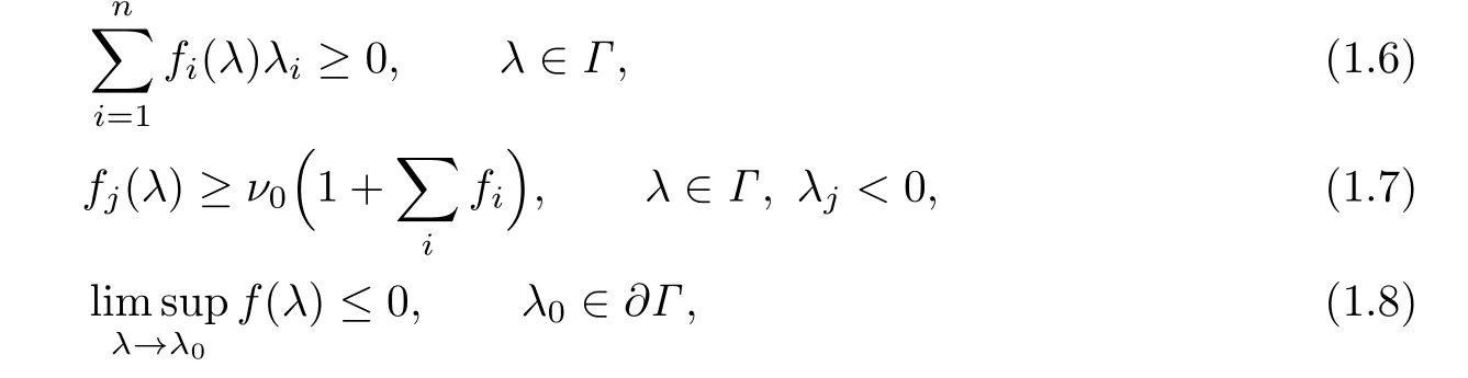
and

where ν0andµ0=µ0(ψ0,ψ1)are some uniform positive constants.

Considering the shape of Ω,we suppose that there exists a sufficiently large constant R such that for every point x∈∂Ω,

where κ1,···,κn-1denote the principal curvatures of∂Ω(related to the interior normal).

Let

Definition 1.1A function v(x,t)is called admissible if v(x,t)∈K.

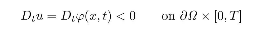
Obviously,for any admissible function u(x,t),the problem(1.1)is of parabolic type.We seek admissible solutions to(1.1)in K;thus we require the given function φ(x,t)to satisfy the following necessary condition:

Theorem 1.1Let α∈(0,1).Suppose thatsatisfies(1.11), Dtφ(x,t)＜0 in,,ψ(x,t)and φ(x,t)satisfy the compatibility conditions up to the first order,∂Ω∈C4and Ω,f,Γ satisfy(1.2)–(1.10). Then the problem(1.1)has a unique admissible solution

Remark 1.1Theorem 1.1 can be used to get the existence of an admissible solutionto the problem(1.1),provided that the problem(1.1)satisfies the compatibility conditions up to the second order,as well as that

To simplify the problem,we assume that for all(x,t)∈Ω×{t=0},

For the function

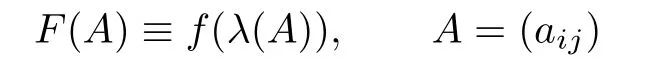
def i ned on the space of n×n symmetric matrices,denote

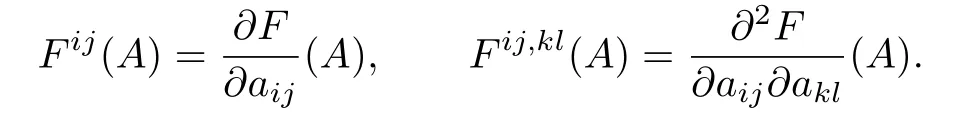
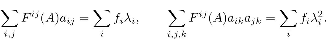
The matrix(Fij)has eigenvalues f1,···,fnand they are positive by(1.2),while(1.3) implies that F is a concave function of A(see[1]).Moreover,we have the following identities (see[3]):

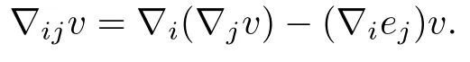
At the end of this introduction we recall some formulae for commuting covariant derivatives on Mn.Throughout the paper,∇denotes the covariant dif f erentiation on Mn.Let e1,e2,···,enbe a local frame on Mn.We use the notations∇i=∇ei,∇ij=∇i∇j,etc. For a dif f erentiable function v defined on Mn,let∇v denotes the gradient,and∇2v the Hessian which is given by

Recall that

and

Finally,from(1.14)and(1.15)we obtain

2 The Existence of Admissible Solutions

We apply the method of continuity to prove the existence of the admissible solutions to the problem(1.1).Actually,we consider a family of problems with parameters τ∈[0,1]:

where u0and ψ0are given in Proposition 2.1 of this paper.Obviously,when τ=1,the problem(2.1)τis just(1.1).

To prove Proposition 2.1,some known results are needed.For the open convex cone Γ in Theorem 1.1,we have

Lemma 2.1[8]Let A,B be real symmetric matrices of order n,and λ(A),λ(B),λ(A+B) be the vectors formed by the n eigenvalues of A,B,A+B,respectively.If λ(A)∈Γ and λ(B)∈Γ,then λ(A+B)∈Γ.

Lemma 2.2[3]Let Ω⊂Mnbe a domain satisfying(1.10).Suppose that there exists a function wsuch that λ(∇2w)∈Γ everywhere.Then there exists a functionwith v=0 on∂Ω and λ(∇2v)∈Γ everywhere.Conversely,∂Ω satisfies(1.10) if there exists a functionwith v=0 on∂Ω and λ(∇2v)∈Γ everywhere.

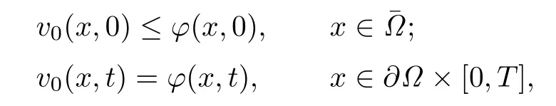
Proposition 2.1There exists a functionsuch that the problem (2.1)0has a solution in K with

Proof.From the necessary condition(1.11)we get λ(∇2φ(x,0))∈Γ for allThen by the assumption that φ(x,t)is smooth we see that there exists a δ∈(0,T)such that

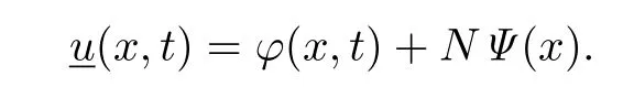
From(1.10)and the proof of Lemma 2.2 in[3],we see that there exists a functionsatisfying λ(∇2Ψ(x))∈Γ,and Ψ(x)≤0 for,Ψ(x)=0 for x∈∂Ω.

Now,let

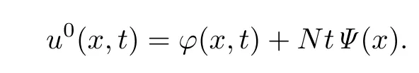
Obviously,

For a fixed t∈[δ,T],

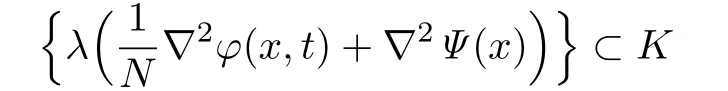
Since{λ(∇2Ψ(x)):x∈}is a compact set in Γ,there exists a compact set K⊂Γ such that

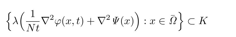
for N large enough.

For a fixed t∈[0,δ],since

we have

by Lemma 2.1.

From the construction of u0,it is easy to get thatand ψ0＞0 on

Proposition 2.1 ensures that the set of the solutions of the one parameter family is nonempty.The existence of admissible solutions to the problem(1.1)would be proved by the continuity method if we have obtained the C2+α,1+α/2estimation of all possible solutions of(2.1)τ(see,for example,[7–8,11]).It is easy to check that the data of(2.1)τand(1.1) have the same property.So it is sufficient to establish an a priori estimation for all possible solutions u(x,t)to(1.1).We do this in the next section.

3 A Priori Estimation Needed

Lemma 3.1Let v(x,t),w(x,t)∈K satisfy the following inequalities:

Proof.Assume that the inequalities in(3.1)are both strict.If the maximum of v-w overis attained on∂pQ,then it is easy to get v≤w inOtherwise,if the maximum of v-w

in some local orthonormal frame on Mn.So the eigenvalues of∇2v are not larger than the corresponding ones of∇2w at the point(x0,t0).

By(1.2),we have

Therefore,

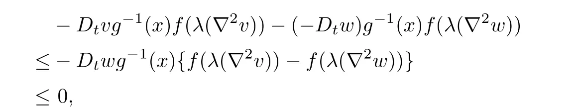
which contradicts(3.1).So v＜w in.In the case of(3.1),for any ε＞0 small enough,let

Then{

By using the result above,it is easy to get vε＜w inSet ε→0.Then we complete the proof.

Theorem 3.1The problem(1.1)has at most one solution in K.

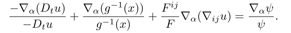
For further usage,we need to rewrite the first equation in(1.1)as

and consider the operator

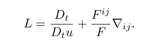
For a fixed u∈K,the operator L is a parabolic one in

Lemma 3.2Let u∈K.If Lv≤0(Lv≥0)in Q for a functionthen

Theorem 3.2There exist positive constants M and m,depending only on the data of the problem,such that for the admissible solution u∈K of the problem(1.1),

Proof.Consider the function

where k is a constant to be determined.Then we have

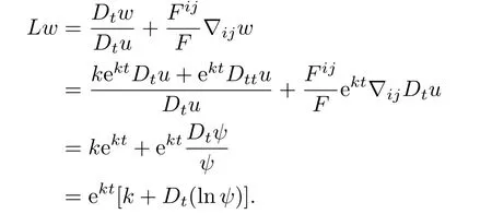
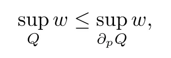
Then Lw≤0.Lemma 3.2 implies

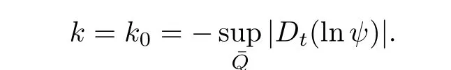
Let

i.e.,

Similarly,let

We get

i.e.,

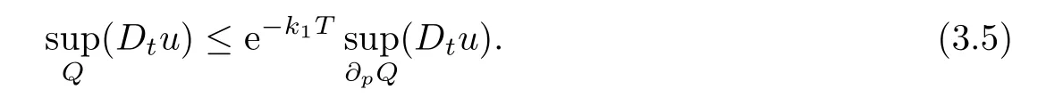
Notice that

and

Then(3.4)and(3.5)yield(3.3).

Theorem 3.3There exists a positive constant M0＞0,depending only on the data of the problem,such that for any admissible solution u∈K of the problem(1.1),

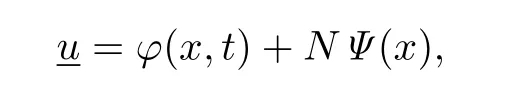
Proof.Let

where N＞0 and is to be determined later,and Ψ(x)is the function given in the proof of Proposition 2.1.Then

i.e.,

Notice that

and λ(∇2Ψ(x))∈Γ,so{λ(∇2Ψ(x)):is a compact set in Γ.Hence there exists a compact set K⊂Γ such that

for an N large enough.Therefore,according to(1.5),we can choose an N sufficiently large such that

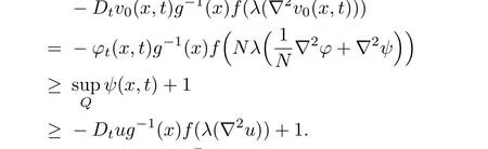
Lemma 3.1 implies v0(x,t)≤u(x,t)in¯Q,which is the lower estimate of u.Also,by the construction of v0,we get

In order to obtain the upper estimate of u,we take the variable t as a parameter.Then we get

Take v1(x,t)to be a harmonic function in Ω with

Then from the comparison principle we get

Thus we can take v0(x,t)and v1(x,t)as the barrier functions to get the bound of|∇u| on∂Ω.

Theorem 3.4Suppose that u∈K is a solution to the problem(1.1).Then there exists a positive constant M1,depending only on the data of the problem,such that

Proof.To derive the interior and global gradient bounds,set

where

and a＞0 is a sufficiently small constant to be determined later.First,we derive a bound for M0when it is attained at an interior point(x0,t0)∈Q.Choose a local orthonormal frame e1,···,enabout x0and dif f erentiate the function lnw+av2which achieves a local maximum at(x0,t0).We obtain that at(x0,t0),

A direct computation shows that

Hence,by(3.11),we have

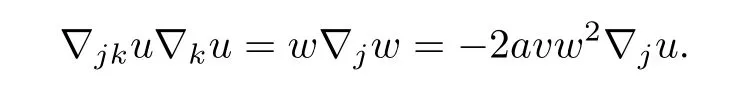
To estimate the term on the right hand side,we dif f erentiate the equation(3.2)to get

By(1.13),we have

According to(3.13),one has

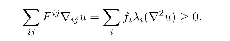
By(3.9),we have

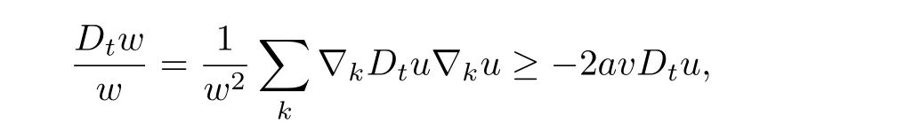
i.e.,

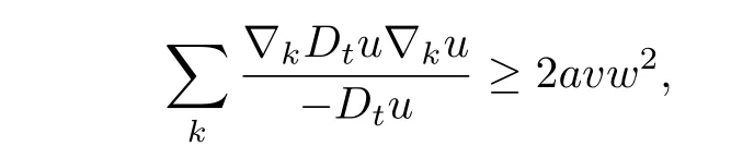
and then(3.14)leads to

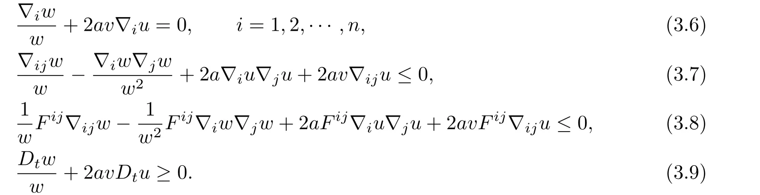
From(3.6)and(3.10),we see that

Combining(3.8),(3.6),(3.12)and(3.15),we obtain

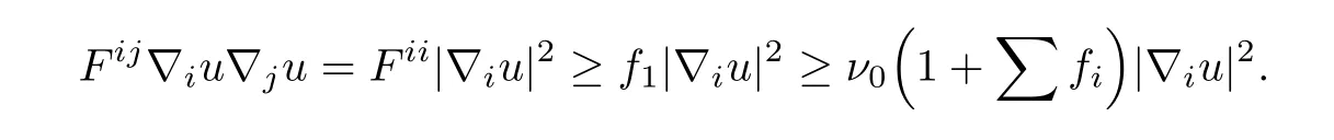
By(1.6),we have

Without loss of generality,we may assume thatis diagonal.Therefore,at,we get

We may also assume that

Then from(3.6)and(3.10)we see that

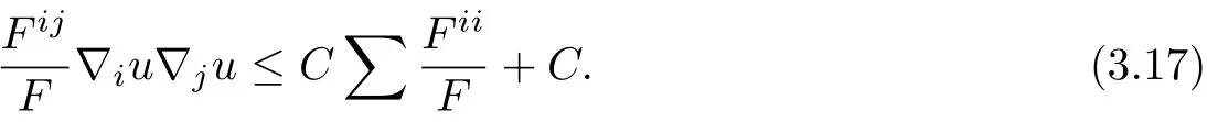
Thus,by(1.7),we have

and

Then,by(3.17),we obtain a bound of|∇1u|and complete the proof.

4 The Bounds for the Second Derivatives

Now we take up an a priori estimate for the second derivative of u.

(a)Bounds for|∇2u|on∂Ω×(0,T].

Rewrite the first equation of(1.1)as

Set

where N＞0 is a constant.Obviously,

so

and

It follows that

For a fixed α≤n,dif f erentiating(3.2)yields

Using the formula for commuting the covariant derivatives,we get

Now consider the distance function

in a small subdomain

Choosing a δ small enough,we may assume that d is smooth in Ωδ.Sinceone has

The following lemma is a direct extension of Lemma 1.2(i)in[13]for the parabolic case.

Lemma 4.1There is a uniform positive constant ε1such that

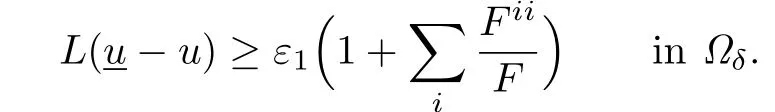
Proof.Consider the function

for ε＞0 small enough.From the concavity of the operator lnf(λ(·))we obtain

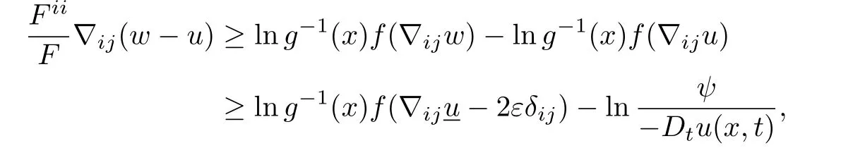
and hence

Notice that

For δ0＞0,let N be large enough so that

i.e.,

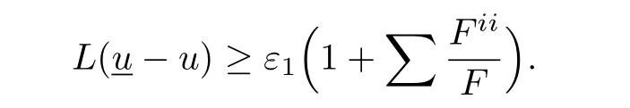
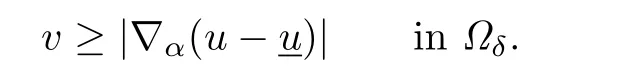
By Lemma 4.1 we may employ a barrier function in Ωδof the form

to estimate∇αnu.By(4.4)and Theorem 3.4,we may choose A≫B≫1 such that

for the mixed normal tangential derivatives∇αnu(x0,t0),α＜n.And we have

since

It follows from the maximum principle that

Consequently,

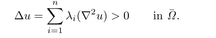
It remains to estimate the double normal derivative∇nnu.Since Δu＞0,we only need to derive an upper bound:

Let Γ′be the projection of Γ to λ′=(λ1,···,λn-1),and D(λ′)be the distance of λ′to∂Γ′for λ′∈Γ′.

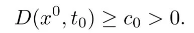
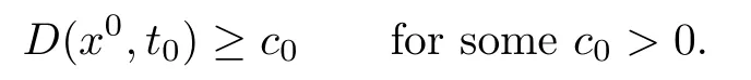
Lemma 4.2For a fixed t0∈(0,T],there exists a uniform constant c0＞0 such that

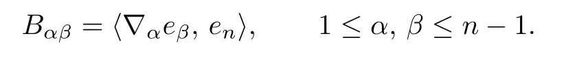
where Π is the second fundamental form of∂Ω.

Proof.Note that for α,β∈TxM with x∈∂Ω,

Consider a point x0∈∂Ω,at which the function D(x,t0)is minimized for x∈∂Ω.It is sufficient to show that

Choose a local orthonormal frame e1,···,enabout x0as before such thatis diagonal and.As in[1],one can f i ndwithµ1≥···≥µn-1≥0,and

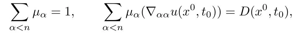
for all x∈∂Ω near x0.Thus by(4.2)we have

for x∈∂Ω near x0.

otherwise we are done.By(4.2)and Lemma 6.2 of[1]we obtain

It follows that

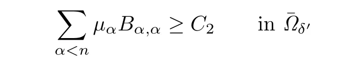
for some uniform positive constants c2andδ,where δ is as in Lemma 4.1.Consequently, by(4.9),

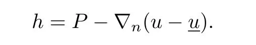
where

Apply Lemma 6.3 of[3]to

Then we obtain

We see that λ(∇2u)(x0,t0)lies in a priori bounded subset of Γ.It thus follows from(1.8) that

for some uniform constant c3＞0.This implies

We are now in a position to prove(4.8).By Lemma 1.2 of[1]and Lemma 4.2,there exists a uniform constant N≫1 such that

Thus,by the strict monotonicity hypothesis(1.2),there exists a constant δ1＞0 such that

This yields a uniform upper bound for∇nnu(x,t0)for x∈Σ,and thus we get

for some uniform constant C1＞0.

(b)Bounds for|∇2u|in

Set

where a＞0,b≥0 are sufficiently small constants to be determined later.It is sufficient to estimate W.

If W is achieved on∂pQ,then W can be estimated via(4.10)and Theorem 3.4.So assume that W is achieved at an interior point(x0,t0)∈Q and for some unit vector ξ∈Tx0Mn. Choose a smooth orthonormal local frame e1,e2,···,enabout x0such that e1(x0)=ξ and{∇iju(x0,t0)}is diagonal.Set λi=∇iiu(x0,t0),i=1,2,···,n.Then we only need to estimate λ1＞0 from above.

At the point(x0,t0)the function ln(def i ned near(x0,t0)) attains its maximum,so we have

and

By(4.12)we have

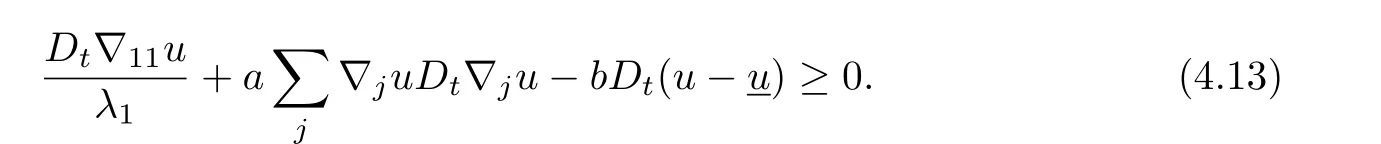
By(4.11)we see that

Add up the two inequalities above we get

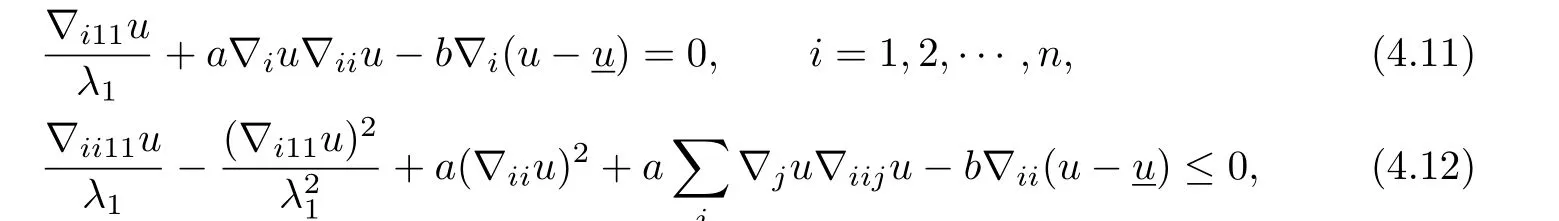
Dif f erentiating(3.2)twice and using the concavity of the function lnf(·),we obtain that at(x0,t0)and for any i,

Thus,(4.14)is transformed into

By(1.2)we have

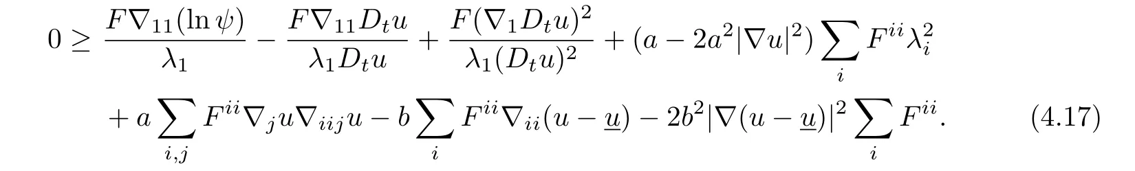
From(4.15)and(4.18)we see that

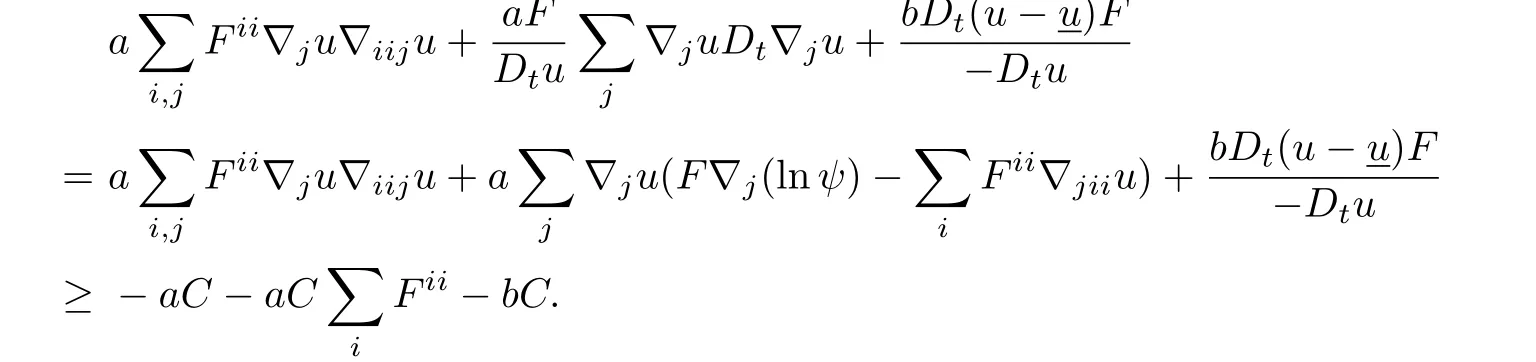
So we can simplify(4.17)into

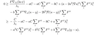
By the proof of Lemma 4.1,there exists a uniform positive constant ε2such that

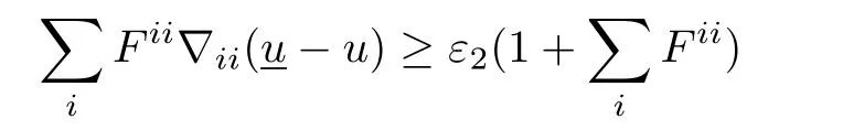
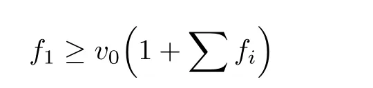
at the point(x0,t0).This yields

We may first choose b＞0 sufficiently small and then choose a≪b to derive from (4.19)that,provided that λ1is sufficiently large.By the arithmeticgeometric mean inequality and assumption(1.9),therefore we obtain

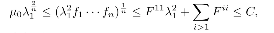
which provides a bound for λ1.

Thus we have proved that the eigenvalues of{∇iju(x,t)}are all bounded and positive for any(x,t)∈Q.On the other hand,we know that these eigenvalues are bounded below from zero by a uniform positive constant by the equation(4.1)and Theorem 3.2.To sum up we have

Theorem 4.1There exist positive constants M2and m2,depending only on the data of the problem(1.1)such that,for the solution u∈K of the problem(1.1),0＜m2＜|∇2u|＜M2in.

Theorem 4.1 implies that(1.1)is uniformly parabolic,and then the desiredestimatefollows from the results of Evans-Krylov theorem.Thus we complete the proof of Theorem 1.1.

[1]Caf f arelli L,Nirenberg L,Spruck J.The Dirichlet problem for nonlinear second-order elliptic equations III.Functions of the eigenvalues of the Hessian.Acta Math.,1985,155:261–301.

[2]Trudinger N S.Weak solutions of Hessian equations.Comm.Partial differential Equations, 1997,22:1251–1261.

[3]Guan B.The Dirichlet problem for Hessian equations on Riemannian manifolds.Calc.Var. Partial differential Equations,1999,8:45–69.

[4]Urbas J.An approximation result for solutions of Hessian equations.Calc.Var.Partial Differential Equations,2007,29:219–230.

[5]Dong H.Hessian equations with elementary symmetric functions.Comm.Partial differential Equations,2006,31:1005–1025.

[6]Ivochkina N M,Trudinger N S,Wang X.The Dirichlet problem for degenerate Hessian equations.Comm.Partial differential Equations,2004,29:219–235.

[7]Ivochkina N M,Ladyzhenskaya O A.The first initial-boundary value problem for evolution equations generated by traces of order m of the hessian of the unknown surface(in Russian). Acad.Sci.Dokl.Math.,1995,50:61–65.

[8]Ren C.The first initial-boundary value problem for fully nonlinear parabolic equations generated by functions of the eigenvalues of the Hessian.J.Math.Anal.Appl.,2008,339:1362–1373.

[9]Wang G,Liu H.Some results on evolutionary equations involving functions of the eigenvalues of the Hessian.Northeast.Math.J.,1997,13:433–448.

[10]Guan B,Li Y.Monge-Amp`ere equations on Riemannian manifolds.J.differential Equations, 1996,132:126–139.

[11]Ren C,Wang G.Parabolic Monge-Amp`ere equation on Riemannian manifolds.Northeast. Math.J.,2007,23:413–424.

[12]Krylov N V.Sequences of convex functions and estimates of the maximum of the solution of a parabolic equation(in Russian).Sibirsk.Mat.Zh.,1976,17:290–303.

[13]Guan B,Spruck J.Boundary value problem on Snfor surfaces of constant Gauss curvature. Ann.of Math.,1993,138:601–624.

35K55,35D05

A

1674-5647(2013)04-0305-15

Received date:Sept.7,2010.

The NSF(11026045)of China.

E-mail address:rency@jlu.edu.cn(Ren C Y).