Modelling the Spread of HIV/AIDS Epidemic

KELATLHEGILE RICARDO GOSALAMANG AND HUANG QING-DAO

(School of Mathematics,Jilin University,Changchun,130012)

Communicated by Li Yong

Modelling the Spread of HIV/AIDS Epidemic

KELATLHEGILE RICARDO GOSALAMANG AND HUANG QING-DAO*

(School of Mathematics,Jilin University,Changchun,130012)

Communicated by Li Yong

In this paper,a deterministic mathematical model for the spread of HIV/AIDS in a variable size population through horizontal transmission is considered. The existence of a threshold parameter,the basic reproduction number,is established, and the stability of both the disease-free equilibrium and the endemic equilibrium is discussed in terms of R0.

spread of HIV/AIDS,horizontal transmission,threshold,stability

1 Introduction

Many recent theoretical,experimental and f i eld studies have challenged the old wisdom that parasites evolve to become harmless to their hosts.Longevity within the host often comes at the expense of other characteristics of evolutionary value to parasites,that is,the spread of replication,transmissibility and resistance to the host's immune response(see[1]). These patterns have also been observed in the context of HIV.The serious consequences of infection with the HIV virus,according to the prevailing view,which is the agent for AIDS, have stimulated many works on the epidemiological implications of this infection(see[2]).

In recent decades,there have been several investigations on infectious diseases using deterministic mathematical models with or without demographic factors(see[3]).Similarly, we investigate in this work,the transmission of HIV,by considering a basic model with three compartments.Determinating the steady state solutions and analysing their stability represent the main part of our analysis,in which we also address the question of whether or not the disease can invade the host population and under what conditions it happens.

2 Model Formulation

We consider a sample of population of size N(t)at time t,with a constant inf l ow rate π of susceptibles.The size N(t)is divided into three subclasses of susceptibles S(t),chronic infectives I(t)and patients who have developed AIDS A(t)with a natural death rate d in each class.The constant progression rate to AIDS is denoted by γ,so thatyears is the mean duration of stay in the compartment I(t).

In this simple HIV model,we assume that the transmission of the disease for the heterosexual population occurs horizontally,that is,due to direct contact.We also assume a homogenous mixing of the population,so the average number of contacts with susceptibles, adequate for the transmission of the infection,of one infective per unit time is given bywhere i=1,2.The incidence rate,the number of new cases,that arise per unit time in this model,is given bywhere the probabilities of transmitting infection from the infective partner to the susceptible partner are given by β1and β2respectively for infectives in compartments I and A.Individuals acquire new sexual partners at a rate c and the average number of adequate contacts of an infective per unit time is given by cβi, i=1,2.The total sexually active population is given by

The transfer diagram is given by Fig.2.1.

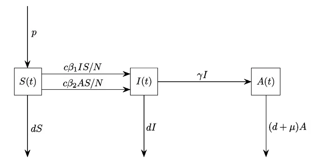
Fig.2.1

The transfer diagram Fig.2.1 leads to the formulation of the autonomous dif f erential system

Adding the equation(2.1)to(2.3)gives

It is easy to see that for the system(2.1)–(2.3),the region

is positively invariant,ensuring that the model is biologically meaningful and well posed.

The model parameters are as follows:

π:constant inf l ow of susceptibles;

d:constant natural death rate;

β1:the probability of transmitting infection from the chronic infective partner to the susceptible partner;

β2:the probability of transmitting infection from the partner who developed AIDS to the susceptible partner;

γ:progression rate to AIDS;

µ:disease-related constant death rate.

3 Equilibria and Reproduction

3.1The Basic Reproduction Number

To calculate the basic reproduction number of the model R0,we employ the technique described in[4].We def i ne the matrix of generation of new infections as

and the matrix of transitions between other states as

We can rewrite the system(2.1)–(2.3)as

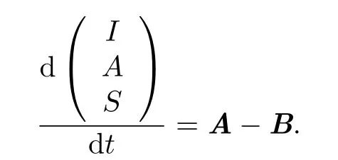
The infected compartments are I and A,given m=2.At the disease free equilibrium(DFE for short)point,

where S*=Using the notations in[4],we have

which gives

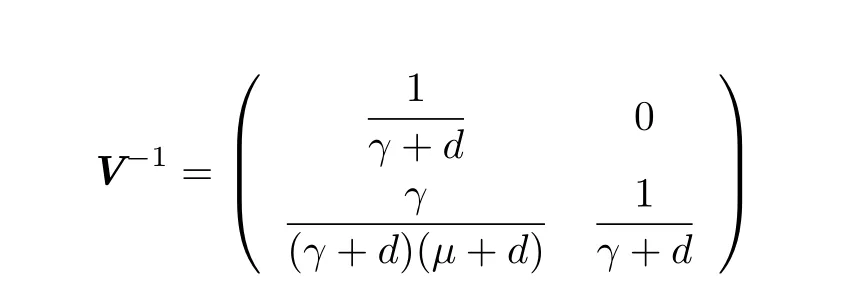
and

The characteristic equation of FV-1is

that is,

The basic reproduction number R0of the model,def i ned as the expected number of secondary cases produced,in a completely susceptible population,by a typical infected individual during its entire period of infectiousness(see,for instance,[5]),is given by the spectral radius(dominant eigenvalue)of FV-1,which is

Remark 3.1Note that if R01≤1 and R02≤1,then

This implies that the epidemic can be contained if each chronic HIV and each AIDS infected individual generates at most one secondary infective.

3.2Steady-state Solutions

In the absence of the disease,the population size approachesas t→∞.Therefore the DEF point is given by.We now derive the coordinates of the endemic equilibrium pointf the system(2.1)–(2.3),i.e.,seek for the solution of

Adding the equation(3.2)to(3.3)yields

and by using(3.4)one obtains

Consequently,one either has

or

where

The solution I*=0 leads to the disease free equilibrium pointWe now consider the solution of(3.7).Substituting R0obtained in(3.1)into(3.7),we have the following equation:

Using the relation

we have

and by(3.4)we get

From(3.5)we have

and by substituting(3.11)into(3.10),we obtain

Substituting(3.12)into(3.9)we obtain

The other solutions can be obtained in terms of R0and are as follows:

Hence the endemic equilibrium point is

Remark 3.2We note that if R0=1,then E1reduces to E0,implying the epidemic clears from the population when R0=1.Also,the endemic equilibrium point of the system (2.1)–(2.3)exists if and only if R＞1.

4 The Stability Analysis of Equilibrium Points

4.1The Analysis of E0

We use the Jacobian of the system(2.1)–(2.3)to analyze the local stability properties of the equilibrium points E0and E1.In the absence of disease,the model has a steady state,called the disease-free equilibrium point.The local stability of E0is then determined based on the signs of the eigenvalues of the Jacobian matrix

The characteristic equation is given by

One of the eigenvalues is λ1=-d and the other two eigenvalues are given by the roots of the quadratic equation

where R0is def i ned in(3.1).This can be written in the form

where

and

It follows that E0is stable if R0＜1 and unstable if R0＞1.The results of the stability analysis can be summarized in the following theorem.

Theorem 4.1The disease-free equilibrium point E0of the system(2.1)–(2.3)is asymptotically stable for R0＜1 and unstable for R0＞1.

We now discuss the global stability of E0.

Theorem 4.2The disease free equilibrium point E0of system(2.1)–(2.3)is globally asymptotically stable for R01≤1 and R02≤1.

Proof.The global stability of the DFE point E0can be proved by taking V=I+A to be a Lyapunov function.Clearly,V=0 is at the DFE point only.The derivative of the Lyapunov function is as follows:

and the equality holds if and only if

And we may conclude that E0is globally asymptotically stable.From a biological point of view,this means that the HIV epidemic dies irrespective of the initial conditions if the average number of infectives generated by a single infective or by a single patient who has developed AIDS is less than one when put in a completely susceptible population.

4.2The Analysis of E1

The Jacobian matrix of system(2.1)–(2.3)at the endemic equilibrium point is given by

where

The cubic characteristic equation is

where

We have R0＞1 at the endemic equilibrium point,and hence b2＞0 since it is a sum of positive terms.

In b1,

since R0＞R01,and hence b1＞0.

Next,we consider b1b2-b0.In this case,all the terms of b2and b1are positive thus giving b1b2-b0＞0 and the two negative terms in-b0are canceled out as follows:

(a)The f i rst term in b2times the fourth term in b1cancels out the f i rst term in-b0as follows:

(b)The second term in-b0is canceled out by the second term in b2times the f i fth term in b1as follows:

Thus b2b1-b0＞0 since it is a sum of positive terms.We have shown that if R0＞1 then b2＞0,b1＞0,b0＞0,and b2b1-b0＞0,showing that the Routh-Hurwitz conditions are satisf i ed.Thus,the endemic equilibrium point is locally asymptotically stable if R0＞1, and we have obtained a proof of the following stability result.The results of the stability analysis can be summarized in the following theorem.

Theorem 4.3The endemic equilibrium point E1of the system(2.1)–(2.3)is asymptotically stable for R0＞1.

Remark 4.1The result on global stability of E0if R01,R02≤1,indicates that the disease clears from the host population irrespective of initial population sizes.The local stability results of the endemic equilibrium point show that the disease persists in the population if the initial population sizes are near the equilibrium state.

5 Numerical Simulations

In this section,we f i rst give estimations of the parameters used in this model and then show several solution curves for cases where R0≤1 and R0＞1.These numerical simulations conf i rm the analytical results and represent a basis which can be compared with future examples in which density-dependent demographics are included.

5.1Parameter Estimates

Table 5.1 shows the parameters that we use in the study and the ranges for those that we choose.At this point we give a brief review of some of the parameters.

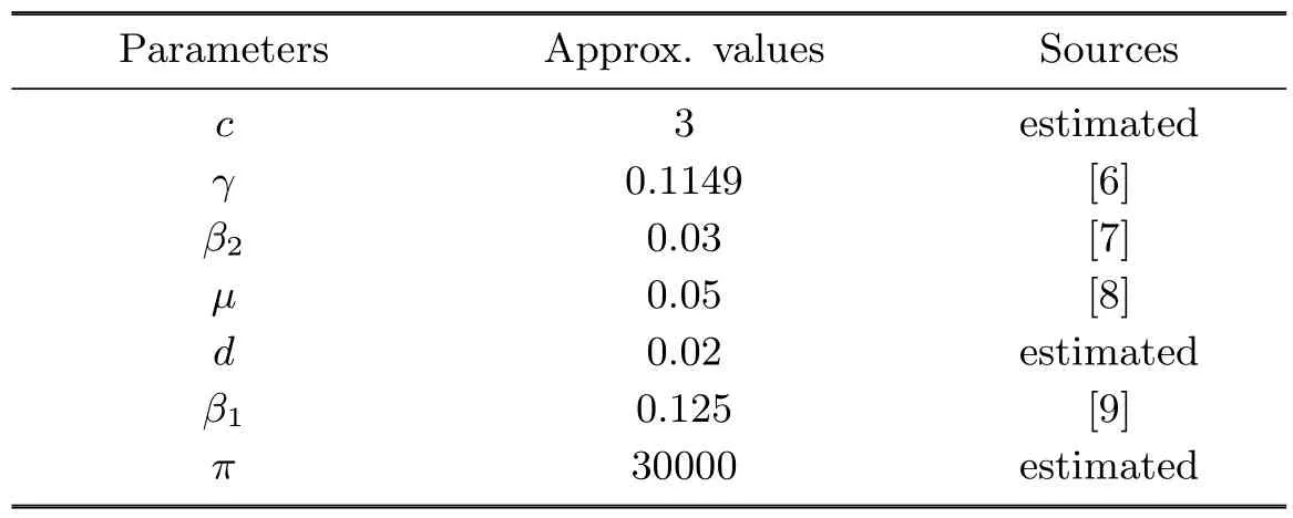
Table 5.1Parameter values,sources

5.2Parameters Common to All Models

Certain parameters are well known and common to dif f erent models,for instance,the removal rate,which is the sum of the natural death rate,d,and the disease related death rate,µ.For the natural death rate,we assume that the individuals in the population are young adults aged 15 years older and above and can be expected to live an average of 50 more years, so d=0.02 yrs-1.[6]approximated the number of years spent in infective groups I and A to be 8.7 years.Hence γ=0.1149 yrs-1.We choose the values of the transmission on probabilities guided by[6].

Fig.5.1 shows the equilibrium susceptible,chronic infected and AIDS populations as functions of R0for the following parameter values:c=3,β2=0.125,β1=0.03,d=0.02, γ=0.1149,µ=0.05 and π=30000.

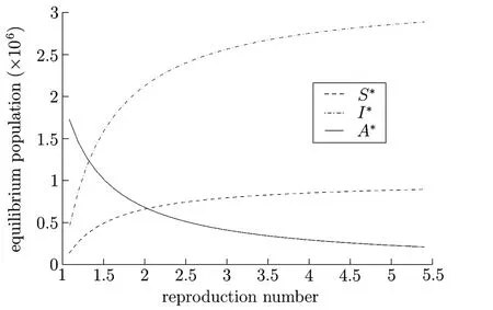
Fig.5.1

From Fig.5.1 we see that as R0increases we have more secondary infection per infective leading to a reduction in the susceptible group and an increase in both the chronic infectives and the AIDS population.The reduction of secondary infections per infective,that is, R0→1,leads to an increase in the population of susceptibles,and reduction in both the infectives and AIDS population which implies that the disease clears of f.

Fig.5.2 shows the dynamics of the model states as time changes for the following parameter values:c=3,β2=0.03,β1=0.125,d=0.02,γ=0.1149,µ=0.05,π=30000and R0=2.5833＞1.

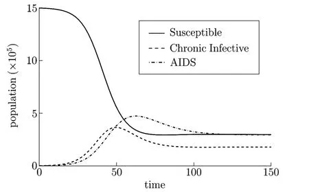
Fig.5.2

Fig.5.2 is a prof i le of the susceptible,chronic infective and AIDS populations for the case R0＞1.The results conf i rm the analytical result in Theorem 4.3.The practical signif i cance of this is that if R0＞1,then the epidemic eventually settles down at an endemic equilibrium point.In this case,there is need to introduce interventions such as treatment and education on behavioral change in order to bring down the infected populations and eradicate the epidemic.

Fig.5.3 conf i rms that as R0decreases towards 1 the epidemic approaches the DFE point, where the plot shows the dynamics of the model states as time changes for the following parameter values:c=3,β2=0.05,β1=0.005,d=0.02,γ=0.1149,µ=0.05,π=30000 and R0=1.2945.

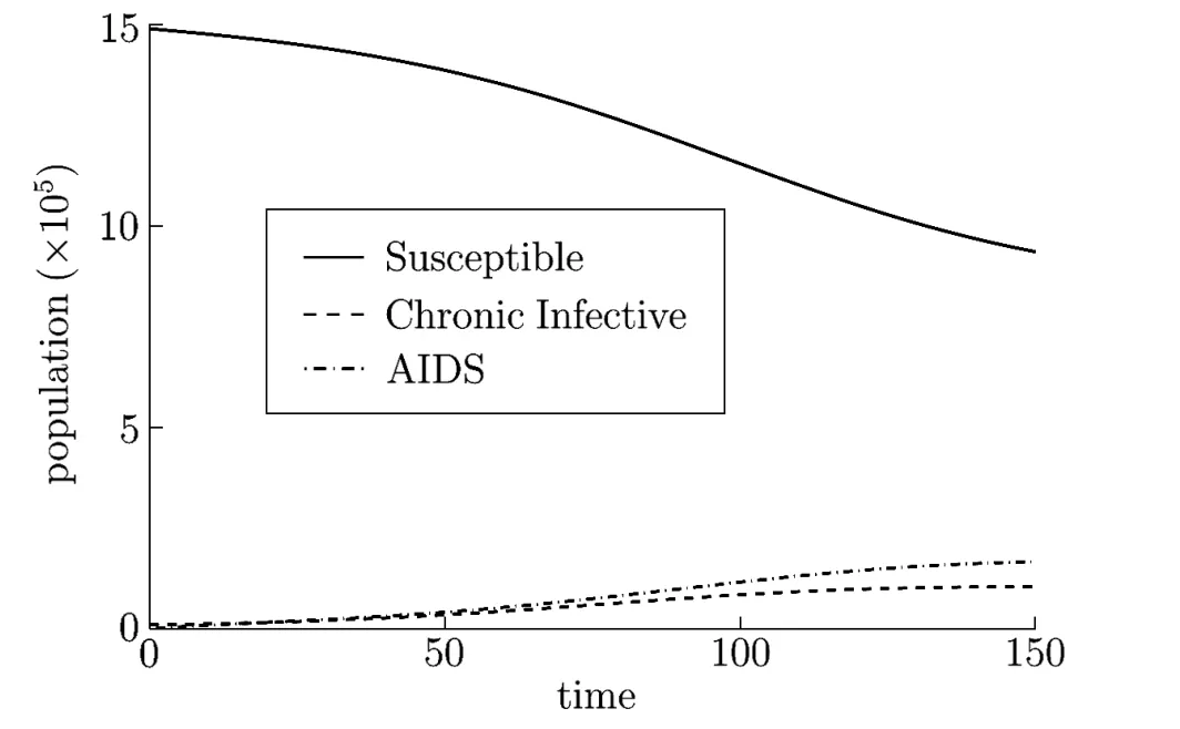
Fig.5.3

The graph depicts that as we reduce the probabilities the epidemic clears.We can see that as time goes on and both the probabilities being small,the disease clears out,and hence the population approaches its carrying capacity K.

6 Conclusion

Mathematical model has now evolved into a useful tool in the area of population dynamics. Its usage has now become a helpful tool especially in combining complex data from various sources in order to analyze equally complex outcomes or results in the system.In this paper our focus was on the spread of HIV/AIDS pandemic by using the average number of people infected when a typical infective enters an entire susceptible population which is known as R0.We found that the signif i cance of R0does not end only on the measuring the burden of the disease but it can also be used to measure the transmission of the disease.

Comparing our model with other models like[10–11]to mention a few,we have both come to a common understanding that if the basic reproduction number R0＜1,the disease free equilibrium is always locally asymptotically stable,in such case the disease does not exist or is eradicated.If R0＞1,a unique endemic equilibrium exists and the disease coexists.We have prove this threshold results which imply that the disease can make the host population goes to extinction if and only if R0＞1,and the burden of the disease can be controlled or reduced or eradicated if and if only R0＜1.When the ratio R0is greater than one it tell us that the spread of the disease is uncontrollable,while R0less than one imply that the disease can be controlled.

AcknowledgementsWe are grateful to Dr Paul Georgescu for his valuable comments and suggestions that led to an improvement of the presentation of the paper.

[1]Lipsitch M,Nowak M A.The evolution of virulence in sexually transmitted HIV/AIDS.J. Theoret.Biol.,1995,174:427–440.

[2]Busenberg S,Cooke K,Thieme H.Demographic change and persistence of HIV/AIDS in a Heterogeneous population.SIAM J.Appl.Math.,1991,51:1030–1052.

[3]Ghosh M,Chandra P,Sinha P,Shukla J B.Modelling the spread of carrier-dependent infectious diseases with environmental ef f ect.Appl.Math.Comput.,2004,152:385–402.

[4]Van den Driessche P,Watmough J.Reproduction numbers and sub-threshold endemic equilibria for compartmental models of disease transmission.Math.Biosci.,2002,180:29–48.

[5]Inaba H.Subcritical Endemic Equilibria in an Age-Duration-Structured HIV/AIDS Epidemic Model.In:Asakura F et al.Hyperbolic Problems:Theory,Numerics and Applications II. Yokohama:Yokohama Publishers,2006:33–40.

[6]Hyman J M,Li J,Stanley E A.The initialization and sensitivity of multigroup models for the transmission of HIV.J.Theoret.Biol.,2001,208:227–249.

[7]Nyabadza F.A mathematics model for combating HIV/AIDS in Southern Africa:will multiple strategies work?J.Biol.Syst.,2006,14(3):357–372.

[8]Kgosimore M,Lungu E M.The ef f ects of vertical transmission on the spread of HIV/AIDS in the presence of treatment.Math.Biosci.Eng.,2006,3:297–312.

[9]Kirschner D.Using mathematics to understand HIV immune dynamics.Notices Amer.Math. Soc.,1996,43(2):191–202.

[10]Gao Q L,Hethcote W H.Disease transmission models with density-dependent demographics. J.Math.Biol.,1992,30:717–731.

[11]Naresh R,Tripathi A,Omar S.Modelliing the spread of AIDS epidemic with vertical transmission.Appl.Math.Comput.,2006,178:262–272.

A

1674-5647(2013)03-0244-11

Received date:April 28,2011.

This work is partly supported by NSF(201115043)of Jilin Province.

*Corresponding author.

E-mail address:gkelatlhegile@yahoo.com(Kelatlhegile R G),huangqd@jlu.edu.cn(Huang Q D).

2000 MR subject classif i cation:92B05