Soft Sensor for Inputs and Parameters Using Nonlinear Singular State Observer in Chemical Processes*
2013-07-31XUFeng许锋WANGYeye汪晔晔andLUOXionglin罗雄麟
XU Feng (许锋), WANG Yeye (汪晔晔) and LUO Xionglin (罗雄麟)**
Research Institute of Automation, China University of Petroleum, Beijing 102249, China
Soft Sensor for Inputs and Parameters Using Nonlinear Singular State Observer in Chemical Processes*
XU Feng (许锋), WANG Yeye (汪晔晔) and LUO Xionglin (罗雄麟)**
Research Institute of Automation, China University of Petroleum, Beijing 102249, China
Chemical processes are usually nonlinear singular systems. In this study, a soft sensor using nonlinear singular state observer is established for unknown inputs and uncertain model parameters in chemical processes, which are augmented as state variables. Based on the observability of the singular system, this paper presents a simplified observability criterion under certain conditions for unknown inputs and uncertain model parameters. When the observability is satisfied, the unknown inputs and the uncertain model parameters are estimated online by the soft sensor using augmented nonlinear singular state observer. The riser reactor of fluid catalytic cracking unit is used as an example for analysis and simulation. With the catalyst circulation rate as the only unknown input without model error, one temperature sensor at the riser reactor outlet will ensure the correct estimation for the catalyst circulation rate. However, when uncertain model parameters also exist, additional temperature sensors must be used to ensure correct estimation for unknown inputs and uncertain model parameters of chemical processes.
soft sensor, state observer, nonlinear singular system, unknown inputs, uncertain model parameters, riser reactor of fluid catalytic cracking unit
1INTRODUCTION
In chemical processes, the operation and control depend on many key input variables that are difficult to measure in real-time with current process instruments. Soft sensor is an effective method for real-time measurement of unmeasurable variables and gradually receives more attention.
At present, the research on soft sensor is mainly on the modeling of soft sensor, establishing mathematical relation between the primary variables unmeasurable and the secondary variables easy to be measured. The modeling of soft sensor includes the extended Kalman filter [1], the high-gain observer [2], the artificial neural network [3], the hybrid fuzzy c-means algorithm and support vector machine [4], the independent component analysis and partial least squares [5], and the relevance vector machine [6]. The multiple model method [7, 8] and local learning adaptive model [9] are also used in the modeling of soft sensor. Because of the complexity and uncertainty of chemical processes, errors are inevitably present. Many input variables are unmeasurable and model parameters are uncertain in chemical processes, so the soft sensor for unknown inputs and uncertain model parameters can be corrected only on-line by secondary variables easy to be measured. The form of soft sensor using output correction of secondary variables will be similar to state observer. When the unknown inputs [10-13] and the uncertain model parameters [14, 15] are augmented as state variables, the soft sensor based on state observer could be built to estimate the unknown inputs and correct the uncertain model parameters online.
The first-principle models of chemical processes are composed of both algebraic and differential equations (DAE), which are called singular systems. Mass and energy balance equations are differential equations, while the equations for mass and energy transfer rate, chemical reaction rate, and thermodynamic state are algebraic equations. In some chemical processes, such as in a riser reactor of fluid catalytic cracking unit (FCCU), the dynamic response of component mass percents is much faster than that of temperature. Hence, the former can be assumed as a quasi-steady state, and mass balance equations become algebraic equations to form another singular system. In the past two decades, singular systems have been widely studied, including stability and Lyapunov theorem [16], poles assignment [17], state feedback stabilization [18], impulse analysis [19], observability and controllability [20-22], most of which focus on linear singular systems or a specific class of nonlinear singular systems. To build the soft sensor for unknown inputs and uncertain model parameters, the nonlinear singular state observer must be used.
State observer for nonlinear singular systems is important in the singular system control theory. The study on the state observer of a linear singular system is mainly focused on the Luenberger observer [23-25] and has been studied intensively. However, state observer for nonlinear singular systems is much more complicated. Zimmer and Meier [26] studied the problem of observing the state of continuous nonlinear descriptor systems in quasilinear form and presented a method to construct a state observer. Lan et al. [27] presented the state observer for bilinear descriptor systems by poles assignment method and the observeerror was Lyapunov asymptotically stable. For a class of Lipschitz nonlinear singular systems, Lu and Ho [28] constructed both types of full-order and reduced-order observers by a unified linear matrix inequality approach. Darouach and Boutat-Baddas gave the sufficient conditions for the existence of observers using linear matrix inequalities formulation [29] and the H∞observers for Lipschitz nonlinear singular systems [30]. Xu et al. [31] transformed a singular system to a normal system after the linearization of nonlinear singular system at current operating point and designed the state observer according to normal system. In this study, we directly design the singular state observer according to singular system. Using the method of adaptive observer [32, 33], the output feedback matrix of state observer is obtained online through poles assignment of the linear parameter-varying singular system at current operating point of the nonlinear singular system.
When unknown inputs and uncertain model parameters are augmented as state variables, state observation will become more difficult as the system dimension increases. Waldraff et al. [34] and Vanden-Berg et al. [35] used the observability matrix of linearized systems to analyse system observability and modified sensor placement.
The present paper presents a simplified observability criterion under certain conditions for unknown inputs and uncertain model parameters. When observability is satisfied, a soft sensor using augmented nonlinear singular state observer is designed for unknown inputs and uncertain model parameters.
2AUGMENTATIONS OF UNKNOWN INPUTS AND UNCERTAIN MODEL PARAMETERS
In the nonlinear singular system given by

x∈Rnis the state, y∈Rlis the measured output, u∈Rm0is the known control input, v∈Rm1is the unknown input, p∈Rm2is the uncertain model parameter, and f(⋅) is the n-dimensional mapping function of the state and is assumed to be smooth. The matrix E∈Rn×nmay be singular, and rank(E)=q<n.
In general real processes, E=diag(Iq,0), and a more practical form is given by

where x1∈Rqis the differential vector and x2∈Rn−qis the algebraic vector.
Chemical processes usually belong to an indexone singular system, which implies that

To be observed, the unknown input v needs to be augmented as state variables. As Besancon [36] reported, the estimation accuracy of an augmented state observer is independent of the dimension of augmented state variables. Thus the dynamic model of augmented unknown input v is

with the initial value v(t0)=v0.
As the uncertain model parameter is constant, it is augmented as a state variable of one dimension and the dynamic model is

with the initial value p(t0)=p0.
After the unknown inputs and uncertain parameters are augmented as state variables, the augmented system becomes

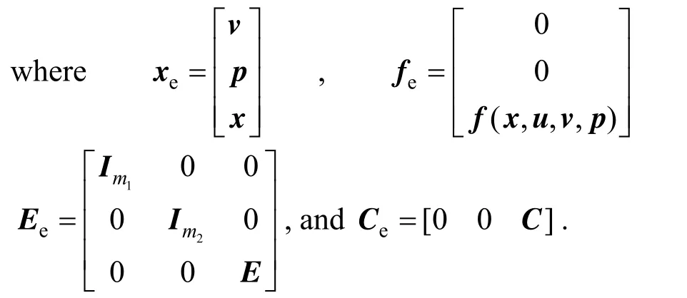
The linearized form of the augmented system in Eq. (5) is


3OBSERVABILITY CRITERION FOR UNKNOWN INPUTS AND UNCERTAIN MODEL PARAMETERS
Based on the observability criterion of singular systems, a simplified observability criterion under certain conditions is presented for unknown inputs anduncertain model parameters.
Lemma 1[37]The linear singular system (E, A, C) is observable, if and only if
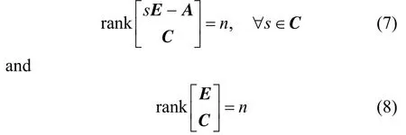
Theorem 1With the assumption that the original system in Eq. (1) is observable at the current operating point, the augmented system in Eq. (5), in which unknown inputs and uncertain model parameters are augmented as state variables, is locally observable at an operating point, if and only if

ProofThe augmented system in Eq. (5) is locally observable at an operating point, if and only if its linearized system ( Ee,Ae,Ce) is observable, such that
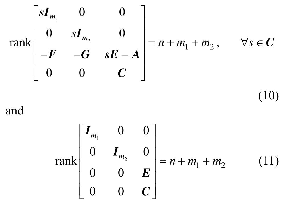
As the original system in Eq. (1) is observable at the current operating point, its linearized system is also observable. Hence, Eq. (11) is obviously satisfied, and Eq. (10) is satisfied, if and only if

This completes the proof.
The necessary observability conditions for unknown inputs and uncertain model parameters can be further deduced fromTheorem 1.
CorollaryThe necessary observability conditions of the augmented system in Eq. (5), in which unknown inputs and uncertain model parameters are augmented as state variables, are

TheCorollarymeans that the augmented system in Eq. (5) will not be observable if the dimension of the unknown inputs plus the dimension of uncertain model parameters m1+m2is larger than the dimension of measured outputs l.
4SOFT SENSOR USING AUGMENTED NONLINEAR SINGULAR STATE OBSERVER
For the augmented system in Eq. (5), a singular state observer exists as

Based on the singular state observer in Eq. (12), a soft sensor is built to estimate the unknown inputs and uncertain model parameters.

where0y is the output of soft sensor,, and

If e=xe−xˆeis the estimation error of real states and estimated states, e satisfies the following error equation of the state observer:

Equation (14) shows that an equilibrium point at e=0 exists. If the error equation in Eq. (14) is locally and asymptotically stable at its equilibrium point e=0, the nonlinear singular state observer in Eq. (12) will be convergent.
The linearized form of the error equation in Eq. (14) at e=0 is

Lemma 2[37]If (E, A, C) is observable, a matrix L always exists, which makes the poles set of (E, A−LC)equal any set Λ of q conjugated complex numbers [i.e., σ(E,A−LC)=Λ].
Theorem 2x=0 is an equilibrium point for the nonlinear singular system Ex˙=f(x) andwhere f:D→Rnis continuously differentiable, and D is the neighbourhood near the origin. If (E, A) is stable and impulse-free, the nonlinear singular system Ex˙=f(x) is asymptotically stable near the origin.
ProofSee Appendix.
Theorem 2extends the theory of Lyapunov linearization and stability from a normal system to a singular system. On the basis ofTheorem 2, the following theorem is proposed for the design of a nonlinear singular state observer.
Theorem 3For the nonlinear singular systemif its linearized system (E, A, C) at the operating point is observable, an asymptotically stable singular state observermust exist.
ProofThe error equation of the singular state observer is

Its linearized form at equilibrium point 0=e is

FromLemma 2, if (E, A, C) is observable, (E, A−LC) can be made stable and impulse-free by choosing L to assign the poles of (E, A−LC) arbitrarily.
FromTheorem 2, if (E, A−LC) is stable and impulse-free, the error equation of the singular state observer is locally and asymptotically stable at 0=e. The singular state observer will be convergent.
This procedure completes the proof.
Hence, if the linearized augmented system (Ee, Ae, Ce) is observable, a singular state observer must exist.
Obviously, the linearized systemic matrix Aeof the augmented system changes with the operating point of the real process, so the feedback gain matrix L of the singular state observer should be adjusted online accordingly to assign the dynamic poles of (Ee, Ae−LCe) at the appropriate location. Therefore, at each sampling time, the feedback gain matrix L should be refreshed to accommodate the operating point changes through online poles assignment of the linearized system.
The implementation steps for calculating the feedback gain matrix L are as follows.
(1) Linearize the augmented nonlinear singular system in Eq. (5) at the operating point to obtain (Ee, Ae, Ce). As Eq. (5) is the index-one singular system, (Ee, Ae, Ce) is the second equivalent form of the singular system [37].

wheree,22A is non-singular,
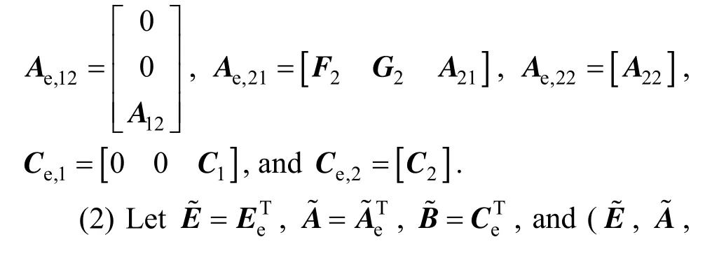

(3) Non-singular matrices Q and P exist.

The system is thus transformed into the first equivalent form of the singular system [37].

(4) As (Ee,Ae,Ce) is observable,is controllable and the slow subsystem (A1,B1) is also controllable. On the basis of the state feedback stabilisation controller design method of the normal system,can be found to assign the poles of (A1−B1K1) at the appropriate locations. Thenmakesfor the designed poles assignments.
(5) With L=KTas the feedback gain matrix of the state observer,

When the state observer is running, changing the feedback gain matrix L is not continuous but discrete. During each sampling period, the feedback gain matrix L remains unchanged, and the state observer will run for a sampling period. After the sampling period is finished, the feedback gain matrix L will be calculated following Steps (1) to (5), and running the next sampling period will begin. For the convergence of numerical simulation, the sampling period h and the poles need to assign λj, j=1,2,…,m1+m2+q which should satisfy the condition
5CASE STUDY
The dynamic model [38] of the riser reactor of FCCU (fluid catalytic cracking unit) is given by

The dynamic model can be rewritten as
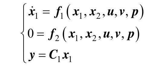
The riser reactor of FCCU is a typical index-one nonlinear singular system. The catalyst circulation rate GCis the main unknown input. The pre-exponential factor of reaction rate constant of crude oil kA0is always influenced by oil material properties and needs to be modified by real process data, which is considered as the main uncertain model parameter. N is the number of FCCU riser segments, and 4N= here.
Firstly, the dynamic model of the FCCU riser reactor is assumed to be accurate without uncertain model parameters, and only GCis unknown. GCis thus augmented as one state variable. Only one temperature sensor is present at the outlet of the FCCU riser, that is

The dimension of the unknown inputs is equal to the dimension of the measurable output, which satisfies the necessary observability condition of theCorollary. At the same time, n=7×N=28, m1=1, m2=1, and

soTheorem 1is also satisfied.
The soft sensor using augmented singular state observer is designed to estimate GC. To examine how the assigned poles of state observer to influence the observation results, we take two set of assigned poles of state observer into account, with the first poles set of [−0.68, −0.68, −0.68, −0.68, −0.68] and the second poles set of [−0.4, −0.4, −0.4, −0.4, −0.4]. To study the influence of signal forms of the unknown input, we consider GCof a square signal or a sinusoidal signal. Fig. 1 (a) shows the curves of the real values and estimated values of GCwhen the unknown input is a square signal, while Fig. 1 (b) shows those when the unknown input is a sinusoidal signal. The estimated values of GCare convergent to the real values. When the assigned poles of state observer are more negative, the convergence rate of state observer is quicker.
To investigate the adaptive capacity for stochastic noise, we add the normally distributed stochastic noise on the signal of the unknown input. Fig. 2 shows the curves of the real values and estimated values of GCwith two poles set for the unknown input of a square signal or a sinusoidal signal with stochastic noise added. The simulation indicates that the impact of stochastic noise is very limited and the state observer with more negative assigned poles is also of the faster convergence rate even under the condition of stochastic noise.
Table 1 shows the mean errors of GCduring the whole dynamic processes of state observer. The mean error with noise is slightly larger than that without noise and the more negative assigned poles gives less mean error.
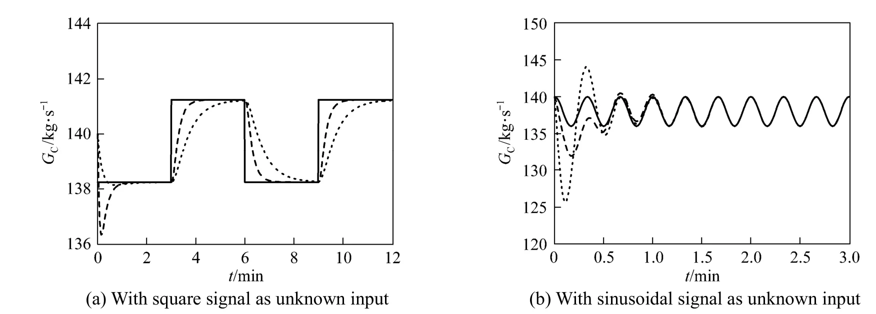
Figure 1Catalyst circulation rate for unknown input without noisereal value; estimated value of the first poles set; estimated value of the second poles set
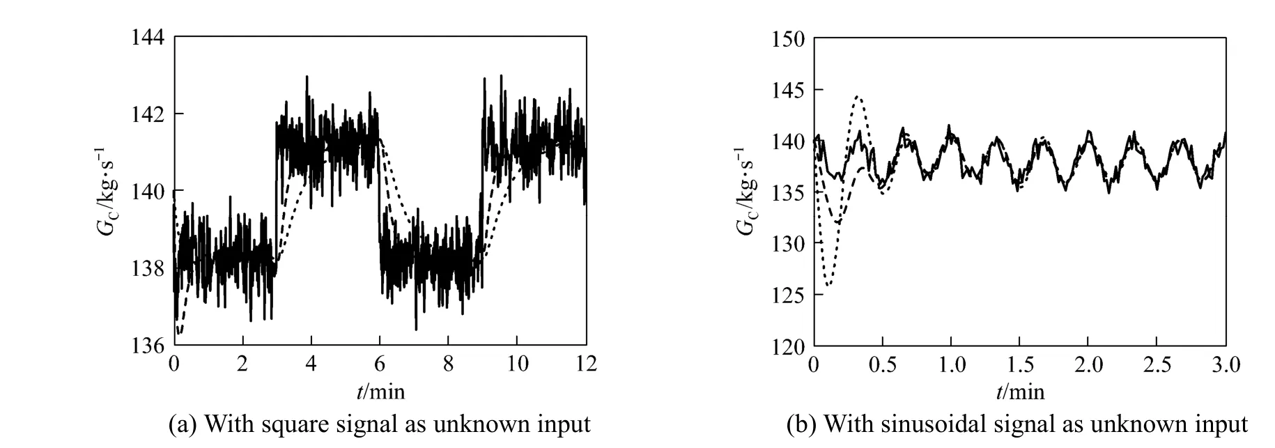
Figure 2Catalyst circulation rate for unknown input with noisereal value; estimated value of the first poles set; estimated value of the second poles set

Table 1The mean errors of the catalyst circulation rate/kg·s−1
Secondly, both unknown input and uncertain model parameter exist in the dynamic model of the FCCU riser reactor, where GCis the unknown input and kA0is the uncertain model parameter. If only one temperature sensor is present at the outlet of the FCCU riser as before, that is C1=[000 1], the dimension of the unknown input plus the dimension of the uncertain model parameter is 2, which is larger than that of measured outputs for the only one temperature sensor at the outlet of the FCCU riser. It will not satisfy the necessary observability conditions of theCorollary. At the same time, n=7×N=28, m1=1, m2=1, and

soTheorem 1is not satisfied either.
More measure points should be added. If one temperature sensor is placed in the middle of the riser reactor and another is at the outlet, the dimension of the measured outputs becomes 2, that is

The dimension of the unknown input plus the dimension of the uncertain model parameter is equal to that of measured outputs. The necessary observability condition of theCorollaryis satisfied. At the same time, n=7×N=28, m1=1, m2=1, and

soTheorem 1is satisfied.
The soft sensor using augmented singular state observer is designed to estimate both unknown input and uncertain model parameter with the temperature sensor in the middle of the riser reactor added. To study the impact of the assigned poles of state observer, we also consider two set of assigned poles of state observer, the first poles set is [−0.7, −0.7, −0.7,−0.7, −0.1, −0.1] and the second set is [−0.5, −0.5,−0.5, −0.5, −0.05, −0.05]. To study the influence of signal forms of the unknown input, we also consider GCof a square signal or a sinusoidal signal. Fig. 3 shows the curves of the real values and estimated values of GCand Fig. 4 shows the curves of kA0. Theestimated values of GCare convergent to the real values, and even if an initial estimation error is encountered for kA0, the estimated value converges to the real value through the online modification of the state observer when it is augmented as a state variable. The assigned poles of state observer are relevant to the convergence rate of state observer. The more negative the assigned poles, the faster the convergence rate.
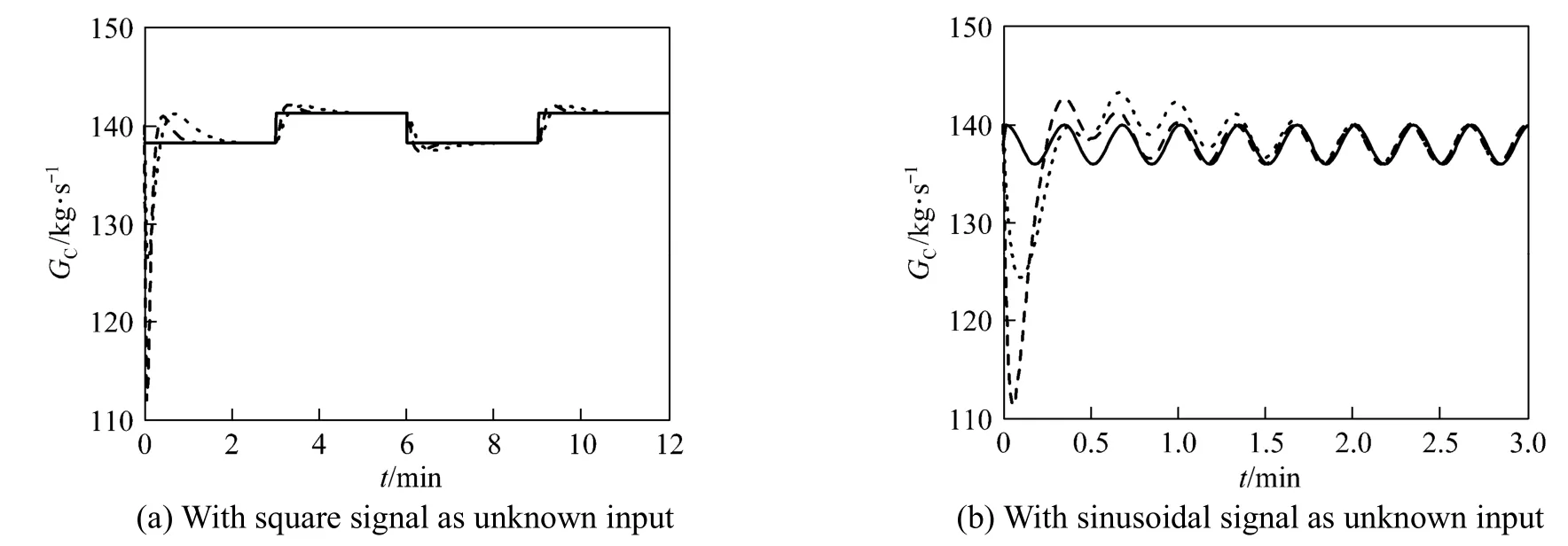
Figure 3Catalyst circulation rate for unknown input and uncertain model parameter without noise real value; estimated value of the first poles set; estimated value of the second poles set

Figure 4Reaction rate constant pre-exponential factor of crude oil without noisereal value; estimated value of the first poles set; estimated value of the second poles set
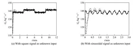
Figure 5Catalyst circulation rate for unknown input and uncertain model parameter with noise real value; estimated value of the first poles set; estimated value of the second poles set
With both the unknown input and uncertain model parameter, we add the normally distributed stochastic noise on the signal of the unknown input. Fig. 5 shows the curves of the real values and estimated values of GCwith stochastic noise and Fig. 6 shows the curves of kA0. The estimated values of GCand kA0converge to the real values and the state observer with more negative assigned poles has faster convergence rate even under the influence of stochastic noise.
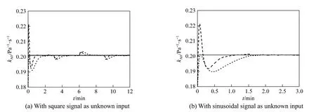
Figure 6Reaction rate constant pre-exponential factor of crude oil with noisereal value; estimated value of the first poles set; estimated value of the second poles set

Table 2The mean errors of the catalyst circulation rate/kg·s−1

Table 3The mean errors of the reaction rate constant pre-exponential factor/10−3Pa−1·s−1
Tables 2 and 3 show the mean errors of GCand kA0in the whole dynamic process of state observer. The mean error with noise is very close to the mean error without noise and the more negative assigned poles also give less mean error. The modified model parameter is used for the online calculation of the state observer, effectively improving the robustness of the soft sensor.
6CONCLUSIONS
For the nonlinear singular system in chemical processes, the unknown inputs and uncertain model parameters are augmented as state variables. On the basis of the observability of the singular system, a simplified observability criterion under certain conditions is presented for unknown input and uncertain model parameters. The augmented system will not be observable if the dimension of the unknown input plus the dimension of the uncertain model parameters is larger than the dimension of the measured output.
When the observability is satisfied, a soft sensor using augmented nonlinear singular state observer is used to estimate the unknown inputs and uncertain model parameters. For the FCCU riser reactor, with only the catalyst circulation rate unknown and no uncertain model parameter, only one temperature sensor at the riser outlet can ensure that the catalyst circulation rate is correctly estimated by soft sensor. When an unknown input and an uncertain model parameter exist, however, another temperature sensor should be added to satisfy the necessary observability condition. Then the catalyst circulation rate and the uncertain model parameter can be estimated correctly by soft sensor.
NOMENCLATURE
A systemic matrix of singular system
B input matrix of singular system
C output matrix of singular system
Cracoke mass percentage of catalyst in riser, %
E singular matrix
EA, Eφreaction activation energy of oil cracking and catalyst deactivation, kJ·kmol−1
e observation error
F unknown input matrix of singular system
FOflow rate of crude oil, kg·s−1
f state equation
G uncertain parameter matrix of singular system
GCcatalyst circulation rate, kg·s−1
ΔHAAcoke adsorption heat, kJ·kg−1
ΔHAR, ΔHDR, ΔHNRcracking reaction heat of crude oil, diesel and gasoline, kJ·kg−1
h output equation
K state feedback gain matrix
kA0, kD0, kN0pre-exponential factor of reaction rate constant of crude oil, diesel and gasoline, Pa−1·s−1
kφ0pre-exponential factor of reaction rate constant of catalyst deactivation, Pa−1
L output feedback matrix of state observer
l dimension of outputs
m dimension of inputs
N number of riser segments
n dimension of states
P, Q equivalent transform matrix
p uncertain model parameter
prapressure of riser reactor, Pa
q rank of singular matrix
R gas constant, 8.314 kJ·kmol−1·K−1
STreaction time, s
Tratemperature of riser reactor, K
u known control input
v unknown input
x state of singular system
y measurable output
yA, yD, yN, yGunconverted oil rate, diesel yield, gasoline yield, gas yield, % (by mass)
y0unmeasurable output
Γ correction coefficient of heat capacity for tube
Λ correction coefficient of heat capacity for oil
υAD, υAN, υAG, υACstoichiometric coefficient of oil-diesel reaction, oilgasoline reaction, oil-gas reaction, oil-coke reaction
υDN, υDG, υDC, υNGstoichiometric coefficient of diesel-gasoline reaction, diesel-gas reaction, diesel-coke reaction, gasoline-gas reaction
ϕ activity of catalyst, %
Superscripts
— the first equivalent form
~ the second equivalent form
^ estimated value
· derivative of time
Subscripts
e augmented system
0 primary variables
1 differential
2 algebraic
REFERENCES
1 Prasad, V., Schley, M., Russo, L. P., Bequette, B. W., “Product property and production rate control of styrene polymerization”, Journal of Process Control,12(3), 353-372 (2002).
2 Bakir, T., Othman, S., Fevotte, G.., Hammouri, H., “Nonlinear observer of crystal-size distribution during batch crystallization”, AIChE Journal,52(6), 2188-2197 (2006).
3 Gonzaga, J.C.B., Meleiro, L.A.C., Kiang, C., Maciel, F.R.,“ANN-based soft-sensor for real-time process monitoring and control of anindustrial polymerization process”, Computers and Chemical Engineering,33(1), 43-49 (2009).
4 Fu, Y., Su, H., Zhang, Y., Chu, J., “Adaptive soft-sensor modeling algorithm based on FCMISVM and its application in PX adsorption separation process”, Chin. J. Chem. Eng.,16(5), 746-751 (2008).
5 Kaneko, H., Arakawa, M., Funatsu, K., “Development of a new soft sensor method using independent component analysis and partial least squares”, AIChE Journal,55(1), 87-98 (2009).
6 Ge, Z., Song, Z., “Nonlinear soft sensor development based on relevance vector machine”, Industrial & Engineering Chemistry Research,49(18), 8685-8693 (2010).
7 Pan, T.H., Wong, D.S.H., Jang, S.S., “Development of a novel soft sensor using a local model network with an adaptive subtractive clustering approach”, Industrial & Engineering Chemistry Research,49(10), 4738-4747 (2010).
8 Li, X., Su, H., Chu, J., “Multiple model soft sensor based on affinity propagation, gaussian process and Bayesian committee machine”, Chin. J. Chem. Eng.,17(1), 95-99 (2009).
9 Kadlec, P., Gabrys, B., “Local learning-based adaptive soft sensor for catalyst activation prediction”, AIChE Journal,57(5), 1288-1301 (2011).
10 Floquet, T., Barbot, J. P., “State and unknown input estimation for linear discrete-time systems”, Automatica,42(11), 1883-1889 (2006).
11 Jiang, Q., Cao, Z., Chen, Z., “Online observation for unmeasurable inputs in FCCU riser”, Journal of Chemical Industry and Engineering,54(2), 204-208 (2003). (in Chinese)
12 Kravaris, C., Sotiropoulos, V., Georgiou, C., “Nonlinear observer design for state and disturbance estimation”, Systems & Control Letters,56(11-12), 730-735 (2007).
13 Ha, Q.P., Trinh, H., “State and input simultaneous estimation for a class of nonlinear systems”, Automatica,40(10), 1779-1785 (2004).
14 Dochain, D., “State and parameter estimation in chemical and biochemical processes: A tutorial”, Journal of Process Control,13(8), 801-818 (2003).
15 Keesman, K.J., “State and parameter estimation in biotechnical batch reactors”, Control Engineering Practice,10(2), 219-225 (2002).
16 Ishihara, J.Y., Terra, M.H., “On the Lyapunov Theorem for singular systems”, IEEE Transactions on Automatic Control,47(11), 1926-1930 (2002).
17 Yu, R., Wang, D., “Structural properties and poles assignability of LTI singular systems under output feedback”, Automatica,39(4), 685-692 (2003).
18 Xia, Y., Boukas, E.K., Shi, P., Zhang, J., “Stability and stabilization of continuous-time singular hybrid systems”, Automatica,45(6), 1504-1509 (2009).
19 Yan, Z., Duan, G., “Impulse analysis of linear time-varying singular systems”, IEEE Transactions on Automatic Control,51(12), 1975-1979 (2006).
20 Ishihara, J.Y., Terra, M.H., “Impulse controllability and observability of rectangular descriptor systems”, IEEE Transactions on Automatic Control,46(6), 991-994 (2001).
21 Wang, C.J., Liao, H.E., “Impulse observability and impulse controllability of linear time-varying singular systems”, Automatica,37(11), 1867-1872 (2001).
22 Reis, T., “Controllability and observability of infinite-dimensional descriptor systems”, IEE E Transactions on Automatic Control,53(4), 929-940 (2008).
23 Hou, M., Muller, P. C., “Observer design for descriptor systems”, IEEE Transactions on Automatic Control,44(1), 164-168 (1999).
24 Wang, W., Zou, Y., “Analysis of impulsive modes and Luenberger observers for descriptor systems”, Systems & Control Letters,44(5), 347-353 (2001).
25 Wang, Z., Shen, Y., Zhang, X., Wang, Q., “Observer design for discrete-time descriptor systems: An LMI approach”, Systems & Control Letters,61(6), 683-687 (2012).
26 Zimmer, G., Meier, J., “On observing nonlinear descriptor systems”, Systems & Control Letters,32(1), 43-48 (1997).
27 Lan, Q., Liang, J., Guo, W., “Design of state observer for generalized bilinear systems”, Systems Engineering and Electronics,29(7), 1144-1148 (2007). (in Chinese).
28 Lu, G., Ho, D. W. C., “Full-order and reduced-order observers for Lipschitz descriptor systems: The unified LMI approach”, IEEE Transactions on Automatic Control,53(7), 563-567 (2006).
29 Darouach, M., Boutat-Baddas, L., “Observers for a class of nonlinear singular systems”, IEEE Transactions on Automatic Control,53(11), 2627-2633 (2008).
30 Darouach, M., Boutat-Baddas, L., Zerrougui, M., “H∞ observers design for a class of nonlinear singular systems”, Automatica,47(11), 2517-2525 (2011).
31 Xu, F., Guan, J., Luo, X., “On-line estimation of FCCU riser unmeasurable variables based on state observer”, CIESC Journal,62(10), 2828-2838 (2011). (in Chinese).
32 Liu, Y., “Robust adaptive observer for nonlinear systems with unmodeled dynamics”, Automatica,45(8), 1891-1895 (2009).
33 Xu, F., Guan, J., Luo, X., “Adaptive state observer design of nonlinear differential-algebraic systems”, Systems Engineering and Electronics,32(11), 2442-2446 (2010). (in Chinese)
34 Waldraff, W., Dochain, D., Bourrel, S., “On the use of observability measures for sensor location in tubular reactor”, Journal of Process Control,8(5-6), 497-505 (1998).
35 VandenBerg, F.W.J., Hoefsloot, H.C.J., Boelens, H.F.M., “Selection of optimal sensor position in a tubular reactor using robust degree of observability criteria”, Chemical Engineering Science,55(4), 827-837(2000).
36 Besancon, G., “Remarks on nonlinear adaptive observer design”, Systems & Control Letters,41(4), 271-280 (2000).
37 Yang, D., Zhang, Q., Yao, B., Singular System, Science Press, Beijing (2004). (in Chinese)
38 Luo, X., Yuan, P., Lin, S., “Dynamic model of fluid catalytic cracking unit (I) Reactor section”, Acta Petrolei S inica (Petroleum Processing Section),14(1), 34-40 (1998). (in Chinese)
APPENDIX
Proof of Theorem 2
Consider a linear singular system described by

where E∈Rn×nis singular, and rank(E)=q<n. r=degdet(sE −A) is assumed, and obviously, r≤q<n. (E, A) is said to be impulse-free if (E, A) is regular and r=q.
Lemma 3[37](E, A) is stable and impulse-free if and only if a matrix Y exists, such that

Theorem 20=x is assumed to be an equilibrium point for the nonlinear singular system ()=˙ Exf x andwhere f:D→Rnis continuously differentiable, and D is the neighbourhood near the origin. If (E, A) is stable and impulse-free, the nonlinear singular system Ex˙=f(x) is asymptotically stable near the origin.
ProofThe origin x=0 is an equilibrium point for the nonlinear singular system [i.e., f(0)=0]. The nonlinear system is linearized near the origin

As (E, A) is stable and impulse-free, V(x)=xTETYx is used as the Lyapunov function for the nonlinear singular system. The derivative of V(x) of the system is given by

FromLemma 3, 0>W can be derived. Thus, the first term on the right of the equation is negative.
Due to the continuous function, g(x) satisfies

Therefore, for any 0γ>, an 0r> exists, such that

Hence,

whereλmin(⋅) is the minimum eigenvalue of a matrix.
As W is symmetric and positive definite, λmin(W) is real and positive., which ensures that V˙ is negative definite. Thus the nonlinear singular system Ex˙=f(x) is asymptotically stable near the origin.
This procedure completes the proof.
10.1016/S1004-9541(13)60570-4
2012-08-28, accepted 2013-01-10.
* Supported by the National Natural Science Foundation of China (21006127), the National Basic Research Program of China (2012CB720500) and the Science Foundation of China University of Petroleum, Beijing (KYJJ2012-05-28).
** To whom correspondence should be addressed. E-mail: luoxionglin@gmail.com
杂志排行
Chinese Journal of Chemical Engineering的其它文章
- A New Tuning Method for Two-Degree-of-Freedom Internal Model Control under Parametric Uncertainty*
- Halloysite Nanotube Composited Thermo-responsive Hydrogel System for Controlled-release*
- Recent Advances in Separation of Bioactive Natural Products*
- A Novel γ-Alumina Supported Fe-Mo Bimetallic Catalyst for Reverse Water Gas Shift Reaction*
- Experimental and Theoretical Studies of CO2Absorption Enhancement by Nano-Al2O3and Carbon Nanotube Particles
- Volumetric and Transport Properties of Aqueous NaB(OH)4Solutions*
