A Nonsmooth Iterative Algorithm for Solving Obstacle Problems
2012-11-14MAGuochun
MA Guo-chun
(College of Science, Hangzhou Normal University, Hangzhou 310036, China)
A Nonsmooth Iterative Algorithm for Solving Obstacle Problems
MA Guo-chun
(College of Science, Hangzhou Normal University, Hangzhou 310036, China)
This paper discussed a numerical method for solving obstacle problems. Discrete problem were obtained by the finite difference method, and an iterative algorithm, which comes from the nonsmooth Newton method with a special choice of generalized Jacobian, for solving the problems was presented. The algorithm is monotonic and will stop in finite steps. The numerical results were listed at the end of the paper.
nonsmooth Newton method; obstacle problem; monotonic algorithm; finite difference method
1 Introduction
Let Ω⊂R2. Consider the obstacle problem: findu∈Ksuch that
(1)
where
(2)
and the obstacle functionψsatisfies the conditionψ∈H1(Ω)∩C(Ω), hereψ≤0 on ∂Ω, the boundary of the domain Ω.
Problem (1)-(2) describes the equilibrium positionuof an elastic membrane constrained to lie above a given obstacleψunder an external forcef∈L2(Ω). This obstacle problem is also called as the lower obstacle problem.
If the solution is smooth enough, then the obstacle problem (1)-(2) is equivalent to the following free boundary problem[1]:
-Δu-f≥0,in Ω1and -Δu-f=0,in Ω2,
(3)
where Ω1={x∈Ω|u(x)=ψ(x)},Ω2={x∈Ω|u(x)>ψ(x)},or equivalently, the complementarity problem:
u-ψ≥0,-Δu-f≥0,(u-ψ)(-Δu-f)=0 in Ω,
(4)
where Ω=Ω1∪Ω2and Ω1∩Ω2=Ø. As usual, Ω1is called the region of contact and Ω2is called the region of non-contact. These two regions in Ω are both unknown.
There are papers solving the obstacle problem by various methods, such as the relaxation projection method[2], the multilevel projection method[3], the multigrid method[4-6], the moving mesh method[7], etc.
For treating the discrete system obtained by the finite element method or the difference method, some algorithms are discussed, see[1,8-10]. Among them, the active set methods are attractive. The active set strategies can be implemented by the multigrid or multilevel techniques[8].
As Gräser[4]said, recently new interest was stimulated by a reinterpretation of the active set approach in terms of nonsmooth Newton methods. M. Hintermüller, V. Kovtunenko, K. Kunisch[11]pointed out a relation between a nonsmooth Newton method and an active set algorithm when they study a kind of constrained quadratic programming problem.
The discretization method we used in the paper is the finite difference method. In the following, for simplicity, we suppose that the domain Ω be a square region and be divided into equalN×Nparts with the step-sizeh=1/Nand nodes (xi,yj),xi=ih,yj=jh,i,j=0,1,2,…,N. Letn=(N-1)2and denote all the inner nodes (x1,y1), (x2,y1), …, (xN-1,y1), (x1,y2), …, (xN-1,y2), …, (xN-1,yN-1) bys1,s2,…,sN-1,sN,…,s2(N-1),…,sn, respectively, following the natural rowwise ordering. If we use the finite difference method with the 5-point scheme to solve the problem (4), then the following generalized complementarity problem is obtained[12]: findU=(U1,U2,…,Un)T∈Rnsuch that
U-Ψ≥0,AU-F≥0, (U-Ψ)T(AU-F)=0,
(5)
where
Ui≐u(si),i.e.,Uiis an approximation ofu(si),i=1,…,n,
Ψ=(ψ(s1),ψ(s2),…,ψ(sn))T,
F=(f(s1)h2,f(s2)h2,…,f(sn)h2)T,
A is the matrix obtained by the finite difference method with the 5-point scheme,
(6)
andEis the (N-1)×(N-1) identity matrix.
This paper aims to solve (5) by solving its equivalent form:
G(U)=max{-AU+F,-U+Ψ}=0,
(7)
where the operator “max” is the componentwise maximum.
In the paper, starting from the nonsmooth Newton method with a special choice of the Jacobian, we deduce an algorithm where the active set strategy is also used for solving the discretized lower obstacle problem (1)-(2). We also give a relation between an active set method and a Newton type method. It is interesting that the algorithm we get is a globally convergent and monotonic algorithm, which has the locally super-linearly convergency and the finite terminating property.
The rest of this paper is organized as follows. In section 2, we will deduce the monotonic algorithm for solving (7) and give the main results of the paper. In section 3, we will prove the main results. In section 4, we will present some numerical results.
2 Algorithms and Main Results
For solving (7), we adapt the following iterative scheme:
(8)
whereU0∈Rnis a suitable initial point and thei-th row vector (Vk)iofVkis computed by
(9)
for eachi=1,2,…,n.
Above iterative method mainly comes from Qi and Sun’s method[13-14], which is called the nonsmooth Newton’s method, and our method computing an element of generalized jacobian of a nonsmooth function[15].
For the iterative scheme (8), we have
Theorem1
1) For any initial pointU0,Vkcomputed by (9) is always nonsingular for eachk≥0, that is to say that each iteration step in (8) is well defined.
2) Supposing thatU*is a solution of (7), the iterative method (8) is locally super-linearly convergent toU*from a suitable pointU0in a neighborhood ofU*.
3) The iterative sequence generalized by (8) is the same as the one generated by the following Algorithm 1, if they use the same initial point.
Algorithm1
Step 0: ChooseU0∈Rnarbitrarily, setk=0.
Step 1: Solve the following equations to getUk+1:
(10)
where
Ik={i|(-Uk+Ψ)i>(-AUk+F)i}∪{i|(-Uk+Ψ)i=(-AUk+F)i,i≠1},
Jk={i|(-Uk+Ψ)i<(-AUk+F)i}∪{i|(-Uk+Ψ)i=(-AUk+F)i,i=1}={1,2,…,n}Ik,k≥0.
(11)
Step 2: Setk=k+1 and turn to Step 1.
Remark1For eachk≥0, although the form of (10) is much simpler than that of (8), we suppose solving the following equivalent form of (10):
(12)
instead of solving (10) directly. The computational cost of solving (12) is lower than that of solving (8) since the scale of the matrixAJk,Jkis smaller than that ofA. As each of the leading principal minors ofAJk,Jkis a principal minor of the positive definite and sparse matrixA[16], so each of the leading principal minors ofAJk,Jkis positive, thereforeAJk,Jkis also positive definite and sparse. Many methods, such as the conjugate gradient method, the pre-conditional conjugate gradient method and the Lanczos method, can be used[17-18]. In the numerical implementation of Algorithm 1, we use the pre-conditional conjugate gradient method[17].
For the convergence of Algorithm 1, we have
Theorem2For eachU0∈Rnchosen arbitrarily, we have
1) Algorithm 1 is always well defined.
2) Algorithm 1 converges locally super-linearly.
3) Algorithm 1 converges globally and monotonically to the solution of (7) and it stops ifIk=Ik+1orUk=Uk+1.
3 Proofs
We need some lemmas first.
Lemma1(The discrete maximum principle, [16]) IfAU≥0, thenU≥0, whereAis defined by (6) andU={U1,U2,…,Un}T∈Rn.
Lemma2LetU={U1,U2,…,Un}T∈RnandA=(aij)n×n∈Rn×nbe a matrix defined by (6). If there exists two disjoint setsIandJsatisfyingI∪J={1,2,…,n}, we have
1) IfUi≥0,∀i∈Iand(AU)i≥0,∀i∈J, thenU≥0.
2) IfU≠0,J≠Ø,Ui=0,∀i∈I,(AU)i≥0,∀i∈J, thenUi=0,∀i∈IandUi>0,∀i∈J.
Proof1) IfJ=Ø, 1) holds obviously. IfI=Ø, 1) is also true by Lemma 1.

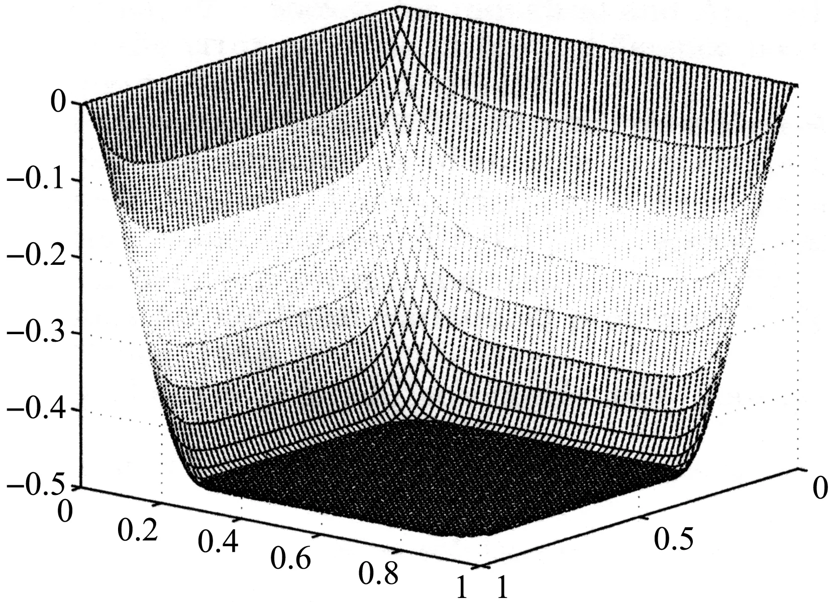
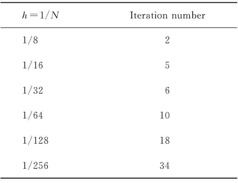
2) SinceUi≥0 is proved for eachi∈Jby 1), it is only needed for us to showUi≠0,∀i∈J.LetJ′={i∈J|Ui>0}, we knowJ′≠Ø becauseU≠0 andUi=0 for alli∈I. Assuming thatJJ′={i∈J|Ui=0}≠Ø, there must existk∈JJ′ such thatUk=0 and one of the following inequalities is true: 0 □ A matrixB=(bij)n×nis called anM-matrix([16]) if bii>0,∀i=1,2,…,n,bij≥0,∀i≠j,Bis nonsingular andB-1≥0. (13) Lemma3(Lemma 4.3.17 in [16]) LetBandCbeM-matrices withC≥B. Then it holds 0≤C-1≤B-1and ||C-1||∞≤||B-1||∞. Lemma4Let the matrixAbe defined by (6) andEbe then×nidentity matrix. For any two setsIandJsatisfyingI∩J=Ø,I∪J={1,2,…,n}, if thei-th row of matrixVI,αis computed by (VI,α)i=αEi, ifi∈Iand (VI,α)i=Ai, ifi∈J, (14) ProofBy Theorem 4.4.1 of [16], the matrixAwith the form (6) is positive definite. IfI=Ø orJ=Ø, thenVI,α=-AorVI,α=-E, 1) and 2) hold obviously. □ TheproofofTheorem11) For eachk≥0, thenVk=-VIk,1according to the construction ofVkin (8) and the definition ofVIk,αin (4). So,Vkis nonsingular for eachk≥0 by Lemma 4 and the nonsmooth Newton method (8) is always well defined. by the properties of semismooth operator, that is to say, the iterative method (8) is locally super-linearly convergent toU*if a suitable pointU0is chosen in a neighborhood ofU*. 3) For eachk≥0, by (9) and the definition of setsIkandJkin (11), the Newton iterative step (8) is equivalent to the following system of equations: (15) which is equivalent to (10). 3) is proved, which completes the proof of the theorem. □ Lemma5For eachU0∈Rnchosen arbitrarily, if the sequence {Uk}k≥0is generated by (8) or by Algorithm 1 andIkandJkare defined by (11) for eachk≥0, then the following hold: 1) The sequence {Uk}k≥1increases monotonically, that is,Uk+1≥Uk,∀k≥1. 2) The sequence {Uk}k≥2is bounded below byΨ, that is,Uk≥Ψ,∀k≥2. 5) For eachk≥2, ifIk≠Ik+1, thenIkIk+1. Lemma 5 can be proved based on the discrete maximum principle. Now, let’s give TheproofofTheorem21) and 2) are the same as the proof of Theorem 1. So to prove the theorem we just need to prove 3). For eachk≥2, by 5) in Lemma 5, for eachU0∈Rn, we haveI2⊇I3⊇…⊇Ik⊇Ik+1⊇…. Since |I2|≤n<+∞, there must exist a numberk, the smallest integer satisfying 2≤k≤|I2|+1≤n+1 such thatIk=Ik+1, by the drawer principle, which deducesUk+1=Uk+2by (10). SinceVk+1(Uk+2-Uk+1)=-G(Uk+1) andVk+1is nonsingular by Theorem 1, we haveG(Uk+1)=0, which means thatUk+1is the solution of (7) and Algorithm 1 stops at thek+1-th step withIk=Ik+1andUk=Uk+1. The arbitration ofU0means that the algorithm is globally. By 1) in Lemma 5, Algorithm 1 is monotonic. 3) is proved. The proof of the theorem is completed. □ In this section, we present a numerical example to show the computational performance of Algorithm 1. All the computations here are performed by MATLAB 7.13. All the programs have been tested at a Dell PowerEdge R71 machine with Intel(R) Xeon(TM) CPU 1.87GHz ×2 and memory 4G. We use the pre-conditional conjunction gradient method[17]to solve each linear system in each iterative step of the algorithm. In the example, we choose 0 as the initial pointU0for Algorithm 1, though it can be chosen arbitrarily. In the programs, we use Dawson’s technique[19], which may be the better technique (see also [15]), to check if two real numbers are equal. Example1[3,9]Let Ω=(0,1)×(0,1), the forcef=-50, the obstacle be a planez=-0.5. Figure 1 shows the approximate solution when the step sizeh=1/64. The interior flat region is the contact region. The numbers of iteration steps are listed in Table 1 for eachh=1/8,1/16,1/32,1/64,1/128,1/256. Fig.1 The solution surface of Example 1 with h=1/64. h=1/NIterationnumber1/821/1651/3261/64101/128181/25634 Thanks Prof. Cheng Xiaoliang and Prof. Huang Zhengda for their help in my researching this work and preparing this paper. [1] Herbin R. A monotonic method for the numerical solution of some free boundary value problems[J]. SIAM Journal of Numeric Analysis,2002,40:2292-2310. [2] Glowinski R. Numerical methods for nonlinear variational problems[C]//Springer Series in Computational Physics. New York: Springer-Verlag,1984. [3] Zhang Yongmin. Multilevel projection algorithm for solving obstacle problems[J]. Computers and Mathematics with Applications,2011,41:1505-1513. [4] Gräser C, Kornhuber R. Multigrid methods for obstacle problems[J]. Journal of Computational Mathematics,2009,27:1-44. [5] Hoppe R H W. Multigrid algorithms for variational inequalities[J]. SIAM Journal of Numerical Analysis,1987,24:1046-1065. [6] Imoro B. Discretized obstacle problems with penalties on nested grids[J]. Applied Numerical Mathematics,2000,32:21-34. [7] Li Ruo, Liu Wenbin, Ma Heping. Moving mesh method with error-estimator-based monitor and its applications to static obstacle problem[J]. Journal of Scientific Computing,2004,21(1):31-55. [8] Kärkkäinen T, Kunisch K, Tarvainen P. Augmented lagrangian active set methods for obstacle problems[J]. Journal of Optimization Theory and Applications,2003,119(3):499-533. [9] Xue Lian, Cheng Xiaoliang. An algorithm for solving the obstacle problems[J]. Computers and Mathematics with Applications,2004,48:1651-1657. [10] Lian Xiaopen, Cen Zhongdi, Cheng Xiaoliang. Some iterative algorithms for the obstacle problems[J]. International Journal of Computer Mathematics,2010,87(11):2493-2502. [11] Hintermüller M, Kovtunenko V, Kunisch K. Semi-smooth Newton methods for a class of unilaterally constrained variational problems[J]. Advanced in Mathematical Sciences and Applications,2004,14:513-535. [12] Cheng Xiaoliang, Xue Lian. On the error estimate of finite difference method for the obstacle problem[J]. Applied Mathematics and Computation,2006,183:416-422. [13] Qi Liqun. Convergence analysis of some algorithms for solving nonsmooth equations[J]. Mathematics of Operations Research,1993,18 (1):227-244. [14] Qi Liqun, Sun Jie. A nonsmooth version of Newton’s method[J]. Mathematical Programming,1993,58:353-367. [15] Huang Zhengda, Ma Guochun. On the computation of an element of clarke generalized jacobian for a vector-valued max function[J]. Nonlinear Analysis: Theory, Methods & Applications,2010,72:998-1009. [16] Hackbusch W. Elliptic differential equations: theory and numerical treatment[M]. Berlin Heidelberg: Springer-Verlag,1992. [17] Barrett R, Berry M, Chan T F,etal. Templates for the solution of linear systems: building blocks for iterative methods[M]. Philadelphia, PA: Society for Industrial and Applied Mathematics (SIAM),1994. [18] Saad Y. Iterative methods for sparse linear systems[M]. Philadelphia, PA, USA: Society for Industrial and Applied Mathematics,2003. [19] Dawson B. Comparing floating point numbers[EB/OL]. (2012-03-20)http://www.cygnus-software.com/papers/comparingfloats/comparingfloats.htm. 一个求解障碍问题的非光滑迭代算法 马国春 (杭州师范大学理学院,浙江 杭州 310036) 讨论了一种求解障碍问题的数值方法.通过有限差分方法得到离散问题,提出了一种源于取一个特殊广义雅可比的非光滑牛顿法的迭代算法.该算法具有单调性和有限步终止性.在文末给出了数值实验. 非光滑牛顿法;障碍问题;单调算法;有限差分法 date:2011-11-30 Supported by NSFC(10731060). Biography:MA Guo-chun(1973—), male, Lecturer, Ph. D., majored in numerical optimization and algorithm analysis. E-mail: maguochun@hznu.edu.cn 10.3969/j.issn.1674-232X.2012.04.002 O241.7MSC201065N06;65F10;65N22;65N12;90C33ArticlecharacterA 1674-232X(2012)04-295-07


4 Numerical Results
Acknowledgements
