Stability-driven Structure Evolution: Exploring the Intrinsic Similarity Between Gas-Solid and Gas-Liquid Systems*

CHEN Jianhua (陈建华), YANG Ning (杨宁)**, GE Wei (葛蔚) and LI Jinghai (李静海)

1 State Key Laboratory of Multi-Phase Complex Systems, Institute of Process Engineering, Chinese Academy of Sciences, Beijing 100190, China

2 Graduate University of Chinese Academy of Sciences, Beijing 100049, China

1 INTRODUCTION

Regime transition is always an important issue in the study of two-phase flow systems. In the earlier studies of fluidization systems, the terminologies of“particulate fluidization” and “aggregative fluidization”were proposed to demarcate two distinct two-phase structures of fluidization states [1, 2]. Mainly due to the density ratio between the continuous phase and dispersed phase, liquid-solid systems are generally considered particulate while gas-solid and gas-liquid systems are aggregative. Compared to the particulate fluidization, more heterogeneous structure emerges in the aggregative fluidization, such as emulsion phase surrounding bubbles (bubbling fluidization) or particlerich clusters and gas-rich dilute broth (fast fluidization).Similarly, more complex structure appears in the heterogeneous (churn) regime of gas-liquid bubbly flow,such as bubble wakes, liquid vortices and coalescence or breakup of bubbles in contrast to the homogeneous regime.

The similarity between gas-solid and gas-liquid flow has been recognized by many researchers [3-6].With increasing gas velocities, gas-solid systems evolve sequentially from uniform expansion, bubbling and turbulent fluidization to fast fluidization and finally dilute transport [7]. These regimes can find their counterpart in gas-liquid systems: dispersed bubbly, coalescing bubbly, churn-turbulent, annular and mist [6],as shown in Fig. 1. If the diameter of apparatus is relatively small, slug flow may be observed between bubbling and turbulent flow. Since design parameters such as pressure drop, heat and mass transfer coefficients are dependent on different flow patterns, a large number of regime maps have been proposed based on experiments and theoretical analysis [8-10]. Bi and Grace [6] found that some empirical approaches or correlations developed for gas-solid fluidization could be used to predict the corresponding transitions between different regimes in gas-liquid bubbly flows.Ellenberger and Krishna [5] proposed a unified approach to scale-up gas-solid fluidized bed or gas-liquid bubble column reactors by analyzing the analogy between these two systems. Analogous to the distinction of dense and dilute phases in bubbling fluidization, the fast-rising bubbles in bubble columns were identified as the dilute phase whereas the liquid phase containing entrained small bubbles as the dense phase. However,these studies have to rely on some empirical correlations, and a more fundamental explanation behind these similarities is still lacking.

Li et al. [11, 12] proposed that the gas-solid fluidized systems belong to a typical dissipative system wherein the two-phase heterogeneous structure is characterized by the so-called dissipative structure. Energy is likely to dissipate in the self-organized and yet heterogeneous ordered structure when the system is far from the equilibrium state. The transition from bubbling to turbulent fluidization can be characterized as a non-equilibrium phase transition,i.e., the first bifurcation point of the gas-solid fluidized system [7]. When the system operates at fast fluidization, global heterogeneous structure may exist, accompanied by the top-dilute phase and bottom-dense phase. The transition from fast fluidization to dilute transport is marked by a jump change (choking), signifying the second bifurcation point of the system. Generally each regime of two-phase flow may correspond to some non-equilibrium steady state, thus the regime transition is essentially a nonequilibrium phase transition.

Hence Li and Kwauk [7] proposed the Energy-Minimization Multi-Scale (EMMS) model which is then extensively developed and applied for gas-solid fluidization in theoretical analysis of regime transition and CFD modeling of gas-solid flow structure [13].The methodology was also extended to other complex systems, in particular, the gas-liquid bubbly flow systems recently [14, 15]. In the EMMS approach, each dominant mechanism was identified and mathematically expressed with an extremum tendency of energy dissipation, and the mutually constrained extremum tendency constitutes a stability condition of the system,reflecting the compromise of different dominant mechanisms. The stability condition can then be used for closing the model in addition to mass and force balance equations. Though the formula of stability condition is system-dependent, it could be used to explore the underlying physics of structure variation with a unified approach.

In this work, we compared the EMMS models for gas-solid and gas-liquid systems to explore the intrinsic similarity of these two systems. The latter is denoted as GL-EMMS model. We confine our discussion in gas-solid fast fluidization and gas-liquid bubbly flow rather than the whole regime expansion. Within the framework of the EMMS model, the solution space of the model is further clarified to help understanding the structure variation during regime transitions.

2 GAS-SOLID FAST FLUIDIZATION

The original EMMS model proposed by Li and Kwauk [7] can be represented in a reduced form in Table 1 [16]. The equations define a non-linear problem for calculating the eight structure parameters to

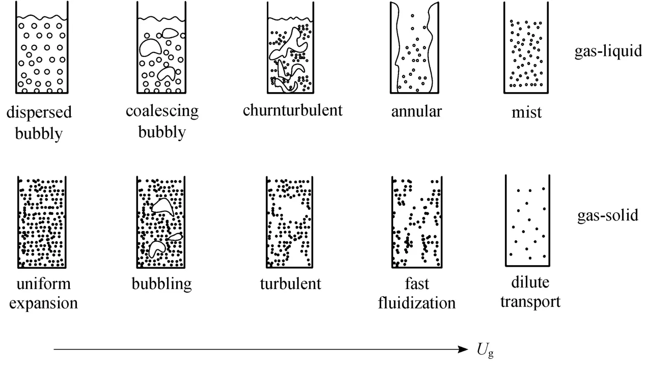
Figure 1 Schematic diagram of regime transition in gas-solid and gas-liquid systems

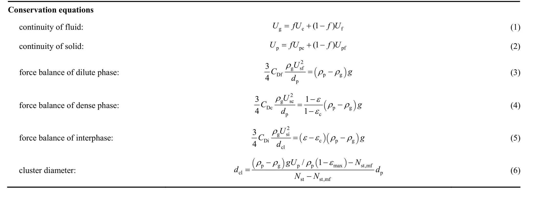
Table 1 The EMMS model for gas-solid systems (Variables: εf, εc,Uf, Uc, Upf, Upc, dcl, f )

Table 1 (Continued)

We noticed two points in the new exploration of the EMMS model. First, the energy dissipation term ofNstat each grid node within the space defined by two structure parameters (εcandf) is independent ofdcl, as can be seen from Eq. (8). Hence we are able to temporarily isolate the variabledcland Eqs. (5), (6) from the whole set of model equations. In other words, with given value ofεc,εfandf, we can immediately obtain the four structure parameters (Uc,Uf,Upc,Upf) from Eqs. (1)-(4). The new algorithm is illustrated in Fig. 2,traversingεcandfover all possible values by small steps. The domain ofεc-fis discretized into 1000×3000 cells, andNstcan be calculated without the need to solve Eqs. (5, 6). Note thatUsicould be obtained from Eqs. (11) and thendclcould also be calculated as an associated variable from Eq. (5) at this moment, but we leave this to the next step. In addition, Eqs. (14) and (15)are used to calculate the parameterUmf.

When searching the whole space of (εc,f), no local minimum ofNstcan be found except at the boundary(see Fig. 3). Hence the second point is to evaluate the effect of the cluster diameter equation on the model solution. It can be seen from Eq. (6) thatdclis a function ofNstandUp, so that the parameterUsican be either determined by Eq. (5) withdclcalculated from Eq. (6), or obtained from its definition formula,i.e.,Eq. (11), withoutdclbeing known in advance. From this viewpoint, Eqs. (5) and (6) provide extra constraints ΔUsi=0 to ensure the model equations converged.

Figure 3 reveals the elaborate structure of the solution space for the EMMS model. The grid nodes(combination ofεcandf), each of which has a valid value ofNst(εc,f) and ΔUsi(εc,f), constitutes a curved surface. The structure parameters at each grid node satisfy the mass and momentum conservative equations for the dilute and dense phases [Eqs. (1)-(4)],but most of them do not obey the cluster diameter correlation of Eq. (6). To let the structure parameters also meeting the force balance equation for interphase(the “phase” between dilute and dense phases) of Eq.(5), the cluster diameterdclhas to be correspondingly adjusted to fit with Eqs. (1)-(4).

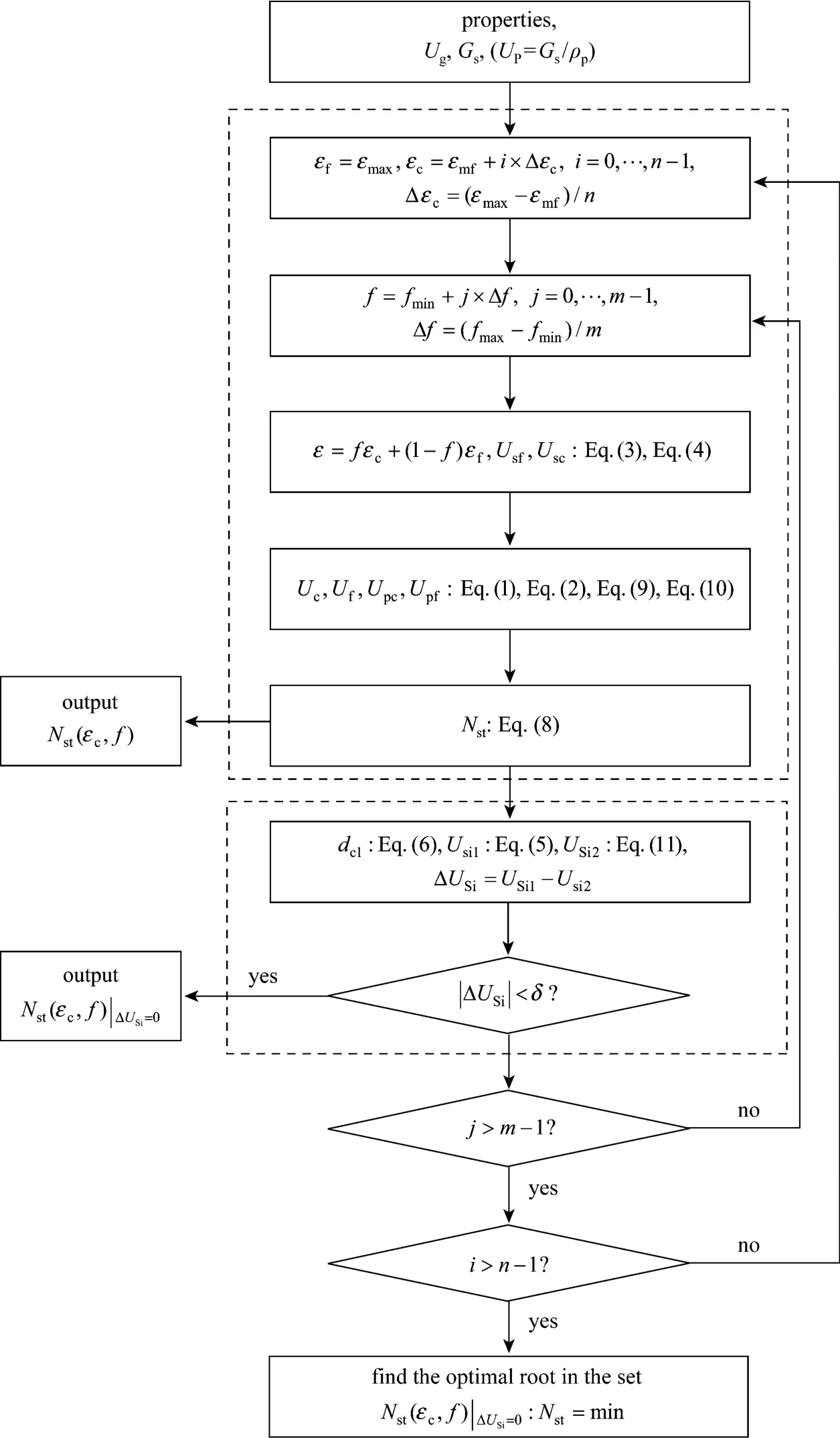
Figure 2 Solution scheme of the EMMS model for gas-solid flow (model equations are in Table 1, m=3000, n=1000)

In this case, the cluster diameter equation, Eq. (6),applies to avoid the adjustment. The characteristic of Eq. (6) lies in thatdclis a function ofUpandNstin contrast to other cluster diameter correlations in literature which is only related to average voidage.Nstis again a combination of other structure parameters.Combination of Eqs. (5), (6) and (11) leads to an extra obeying the conservative equations of dense and dilute phases [Eqs. (1)-(4)], to a curve also satisfying the cluster diameter correlation and the force balance equation for the interphase [Eqs. (5), (6)], and finally shrinking into the points with the minimum ofNst.

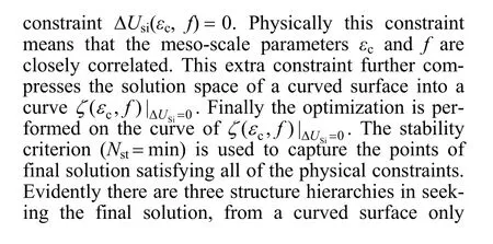
Figure 4 illustrates the solution curves of differentUgat a constant solid flow rateGs=50 kg·m-2·s-1.There are one or two points of the minimum ofNstfor each curve. This can be more clearly identified from Fig. 5 in which the solution space is projected on theNst-εcplane. The boundary ofεc=εmfis considered as a local minimum ifNst(εmf)＜Nst(εmf+ Δεc). Another local minimum ofNstmay appear at a highεcdenoted asεo. With decreasingUg, a state ofNst(εmf)=Nst(εo)can be achieved, signifying the regime transition from dilute transport to fast fluidizationt [16, 17]. This transition is well known as the “C type” choking [18].More details about choking can be found in the references [18, 19]. Before chokingNst(εo) is always smaller thanNst(εmf) and the former is the real solution of the system, as shown in Fig. 5. After chokingNst(εmf) becomes the smaller one. The global minimum point shifts between the two local minima when choking happens. There is a large difference for dense phase structure parameterεcbefore and after choking, which agrees with the experimental evidence that choking is a collapse of suspension with decreasingUgor increasingGs[20].

Figure 4 The solution spaces of different Ug at constant solid flow rate (Gs=50 kg·m-2·s-1)

The bifurcation phenomena can be understood from Fig. 6. With increasingUg, the two local minima ofNstgenerate two branches, and one of them should be a pseudo solution. The branch 1-1 in Fig. 6 (a) corresponds to the local minimum ofNstwhenεc=εmfand the branch 1’-1’ in Fig. 6 (b) is an associated curve of branch 1-1 because all the structure parameters are determined by the stability criterion. The branches 2-2 and 2’-2’ correspond to the other local minimum withεc=εo. The stability criterion requires the global minimization ofNst, so the real solution shifts from branch 1-1 to branch 2-2 at the transition point. Correspondingly the voidage curve shifts from 1’-1’ to 2’-2’ and this jump change reflects the abrupt change in the phase structure. As a result, the solid line in Fig. 6 shows the real solution and the broken line represents the pseudo solution.

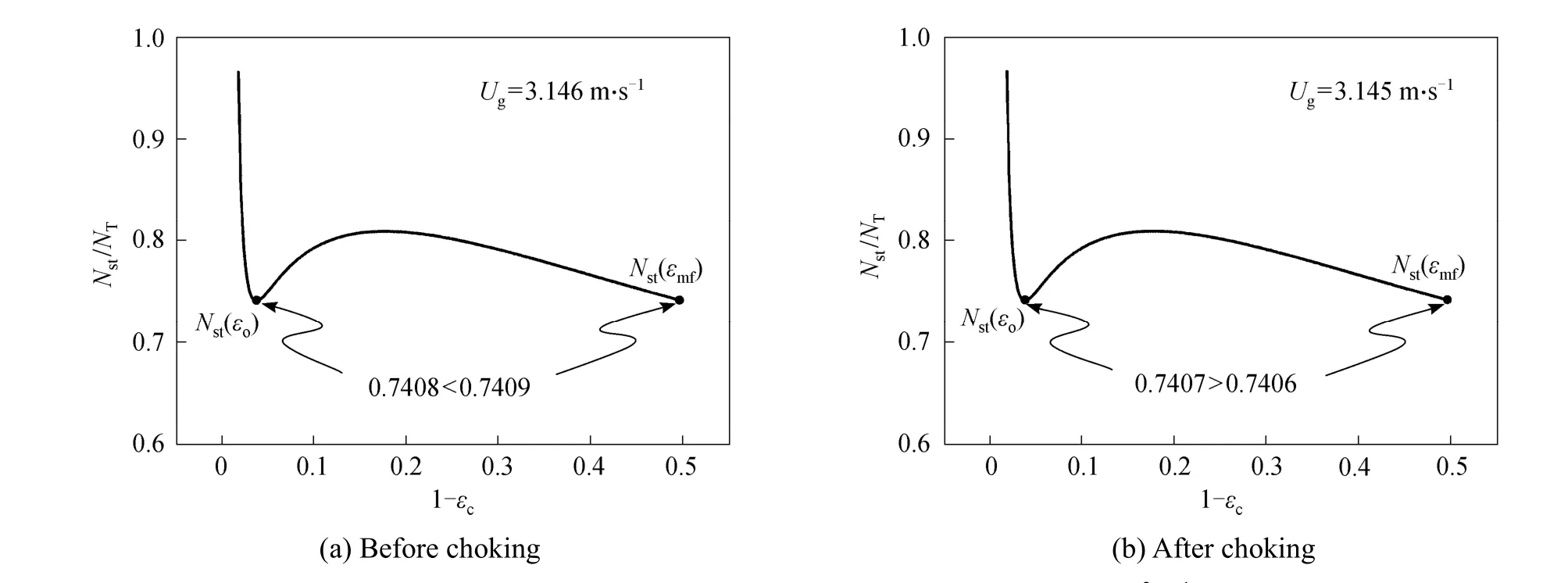
Figure 5 The two local minima of Nst/NT [16] (Gs=50 kg·m-2·s-1)

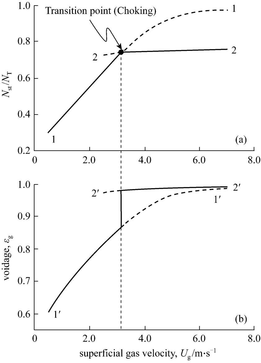
Figure 6 Relationship between structure bifurcation and energy dissipation in gas-solid system

Liet al. [17, 21] recognized that the bifurcation phenomena should relate the structure variation of the system to the stability condition which physically reflects the compromise of two different mechanisms:the tendency of gas passing through particle layer with the least resistance (Wst=min) and the tendency of particles maintaining least gravitational potential (ε=min).But in general neither the gas nor the particles dominate the system, and the former gas-dominated and the latter particle-dominated mechanisms coexists in the system and jointly leads to the stability condition{Nst=Wst/[ρp(1-ε)]}.

The new findings in this study on the hierarchy of solution structure and the description of the structure evolution using the two branches of voidage andNstwould further reinforce the understanding of the essence of the EMMS model. In recent years there is some work in the literature on the modification of cluster diameter correlations of the EMMS model [22].This work also suggests that the cluster diameter correlation be physically related to the meso-scale energy dissipation reflecting the compromise between different dominant mechanisms, and be mathematically of a curve with two local minima when intersecting with the curved surface of Fig. 3. The latter guarantees the co-existence of the bi-stable states of the system when regime transition occurs.

3 GAS-LIQUID BUBBLY FLOW

Our previous work [23-25] established the Dual-Bubble-Size (DBS) model, extending the EMMS method to gas-liquid bubbly flow. The system structure is resolved into a liquid phase, a small bubble phase and a large bubble phase. Six structure parameters are used to describe the system,i.e., bubble diameterdSanddL, gas volume fractionfSandfL, superficial gas velocityUg,SandUg,L. The total energy dissipation rate per unit mass is resolved to three parts:energy dissipation due to bubble oscillationNsurf, viscous dissipation in liquid phaseNturband energy dissipation due to bubble breakageNbreak. The stability criterion is proposed as the minimization of microscale energy dissipation terms (ΣNsurf,i+Nturb). The model equations are summarized in Table 2.

There are six structure parameters and only threeconservation equations in the model, thus three variables are open. Each conservation equation can be considered as a constraint. Analogous to the solution strategy of the EMMS model for gas-solid systems,the non-linear optimization problem is solved by searching the space of open structure parameters to locate the minimum points of the microscale energy dissipation (ΣNsurf,i+Nturb). Fig. 7 shows the solution scheme of the GL-EMMS model in the air-water system.dS,dLandUg,Sare selected as three open variables to construct the solution space. In this work, the minimum bubble diameter is set as 0.5 mm and the maximum bubble diameter as 60 mm. Since the global minimum of (ΣNsurf,i+Nturb) is always attained in the medium value of bubble diameters, the real solution is independent on the minimum and maximum bubble diameters. The logarithmic steps fordSanddLare used to capture sufficient information of structure variation at small bubble region. The grid partition ofm×n×lis performed as 55×55×100 considering the balance between computation load and numerical precision.

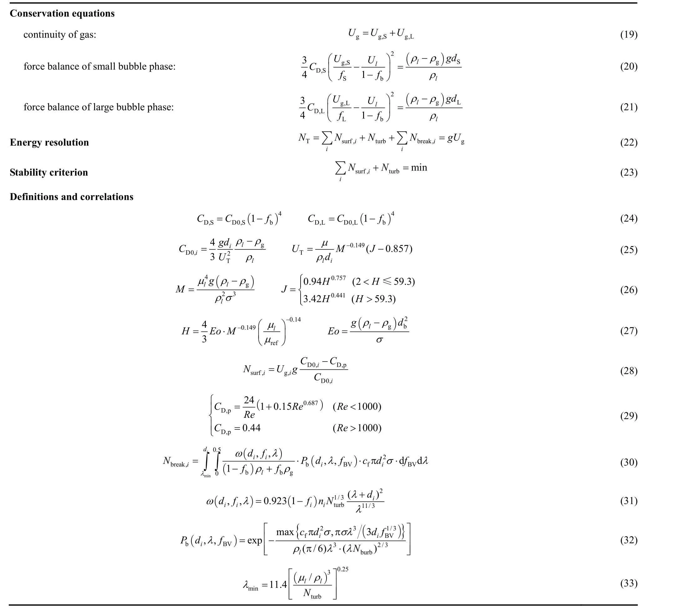
Table 2 The EMMS model equations for gas-liquid flow (GL-EMMS) (Variables: Ug,S, Ug,L, dS, dL, fS, fL)

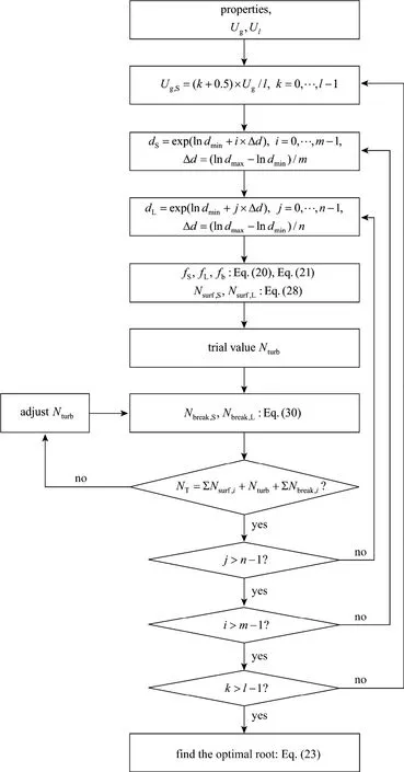
Figure 7 Solution scheme of the GL-EMMS model for gas-liquid systems

The GL-EMMS model is capable of predicting the regime transition from homogeneous and transitional flows to heterogeneous flow between 0.128 m·s-1and 0.129 m·s-1for air-water system, as found by many experiments [26-28]. Fig. 8 shows the solution space for these two gas velocities. Two troughs can be clearly seen in the solution space. In other words, there are also two local minima of the stability condition, which is analogous to the case in the gas-solid systems (see Fig. 5). When regime transition occurs, the global minimum point shifts fromdS=1.42 mm todS=2.86 mm while the large bubble diameter remains to be 8.85 mm. Fig. 9 depicts the stability criterion againstdSonly and the red points mark all possible solutions with respect toUg. There is only one local minimum at lower gas velocities. When the second local minimum appears the system may fall into a bi-stable state as that in gas-solid systems. Note that the jump change point could be more accurately captured by fining the grid resolution and optimizing the solution algorithm [29].

The bifurcation is related to the compromise between two dominant mechanisms in gas-liquid systems: the ability of gas playing the leading role in pattern formation through the minimization of energy dissipationvialiquid viscosityNturb, and the ability of liquid through the minimization of energy dissipation due to the response of bubble surface to liquidNsurf.

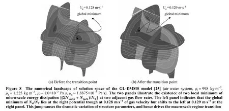
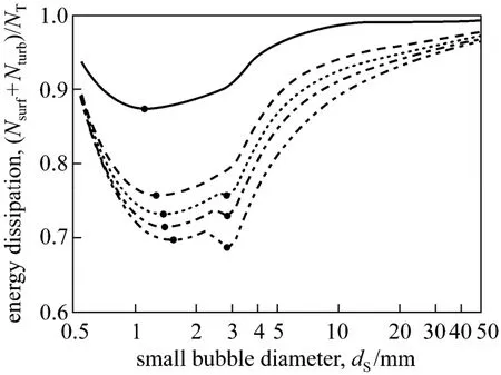
Figure 9 Variation of energy dissipation against small diameter with increasing gas velocity (the points mark the local minima)superficial gas velocity/m·s-1: 0.02; 0.06; 0.08;0.10; 0.14

Analogous to the bifurcation for gas-solid systems, two branches can also be found for gas-liquid systems, as illustrated in Fig. 10. They are determined by the local minima of micro-scale energy dissipation within the solution space of structure parameters for each gas velocity. The solid line denotes the real solution and the broken line denotes the pseudo solution.The two branches in Fig. 10 (a) are continuous, even at the crossing point; but discontinuity occurs on the gas hold-up curve. This characteristic is coincident more or less with first-order phase transition in equilibrium thermodynamics which obeys the principle of minimization of the Gibbs free energy. When the first-order phase transition happens, the Gibbs free energy exhibits continuity but its first derivative such as the specific volume exhibits discontinuity. Note that the regime transition in two-phase flow and the firstorder phase transition in thermodynamics are of different physical implications, because the former belongs to a non-linear non-equilibrium thermodynamics problem; whereas the latter is always regarded as an equilibrium system. The analogy discussed herein is purely from the view of numerical characteristics.

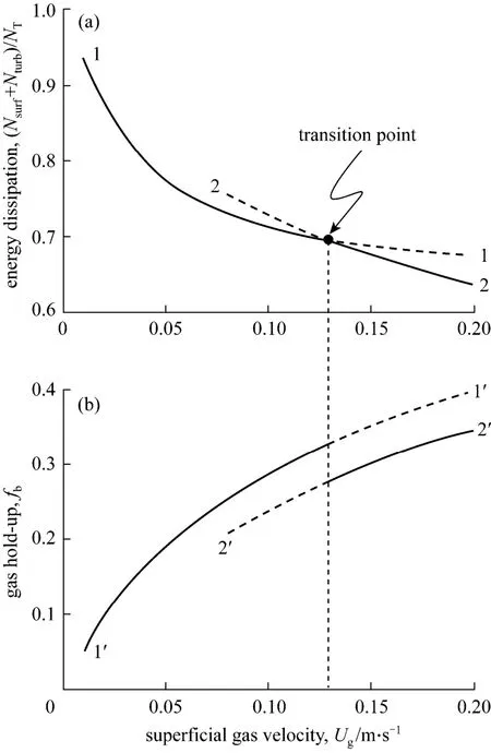
Figure 10 Relationship between structure bifurcation and energy dissipation in bubble columns [14]

4 CONCLUSIONS

This work attempts to analyze the intrinsic similarity between gas-solid and gas-liquid two-phase flow systems within the framework of the EMMS approach. The models solution spaces for the two systems are exhaustively analyzed, and thus regime transitions in gas-solid fluidization and gas-liquid bubbly flows can be theoretically predicted under an unified modeling strategy. For gas-solid systems, the cluster diameter is found to provide an extra constraint on the final solution, and hence critical to capturing the bi-metastable states and the regime transition. The bifurcation of minimized energy dissipation rate can be clearly observed by recording all local minima of stability criterion in the solution space, reflecting the compromise between two different mechanisms. Regime transition is therefore attributed to the existence of the multiple stable states captured in the numerical solution. The relationship between the bifurcations of stability conditions and of structure parameters is found to exist in both gas-solid and gas-liquid two-phase flow systems, indicating that the stability conditions,though system-dependent in expression, is the drive for the structure evolution of the systems. The new findings on the three hierarchies of solution structure in the model and the similar bifurcations in gas-solid and gas-liquid systems would further reinforce the understanding of the essence of the EMMS approach.

NOMENCLATURE

CDdrag coefficient for a bubble swarm

CD0drag coefficient for a bubble in quiescent liquid

cfcoefficient of surface area increase [cf=(fBV)2/3+ (1 - fBV)2/3-1]

dbbubble diameter, m

dclcluster diameter, m

dLlarge bubble diameter, m

dpparticle diameter, m

dSsmall bubble diameter, m

Eo Eötvos number

f volume fraction of dense phase

fBVbreakup ratio of daughter bubble to its mother bubble

fbvolume fraction of gas phase

fLvolume fraction of large bubbles

fSvolume fraction of small bubbles

Gssolid flow rate, kg·m-2·s-1

g gravity acceleration, m·s-2

M Morton number

Nbreakenergy dissipation rate due to bubble breakage and coalescence per unit mass, m2·s-3

Ndenergy dissipation due to collision and friction per unit mass,m2·s-3

Nstenergy dissipation rate for suspending and transporting particles per unit mass, m2·s-3

Nsurfenergy dissipation rate due to bubble oscillation per unit mass,m2·s-3

NTtotal energy dissipation rate per unit mass, m2·s-3

Nturbenergy dissipation rate in turbulent liquid phase per unit mass,m2·s-3

ninumber density of bubbles, m-3

Pbbubble breakup probability

Ucsuperficial gas velocity in dense phase, m·s-1

Ufsuperficial gas velocity in dilute phase, m·s-1

Ugsuperficial gas velocity, m·s-1

Ug,Lsuperficial gas velocity for large bubble phase, m·s-1

Ug,Ssuperficial gas velocity for small bubble phase, m·s-1

Ulsuperficial liquid velocity, m·s-1

Upsuperficial solid velocity, m·s-1

Upcsuperficial solid velocity in dense phase, m·s-1

Upfsuperficial solid velocity in dilute phase, m·s-1

Usslip velocity, m·s-1

Wstvolume specific energy consumption for suspension and transportation of particles, W·m-3

β drag coefficient for a control volume, kg·m-3·s-1

ε local average voidage

λ character size of eddy, m

μ viscosity, kg·m-1·s-1

ρ density, kg·m-3

σ surface tension, N·m-1

ω collision frequency, s-1

Subscripts

b bubble

c dense phase

f dilute phase

g gas

i interphase

i represents “S” and “L” for small, and large bubble phase, respectively

L large bubble phase

l liquid

min minimum

mf minimum fluidization

max maximum

p particle

S small bubble phase

1 Wilhelm, R.H., Kwauk, M., “Fluidization of solid particles”, Chem.Eng. Prog., 44, 201-218 (1948).

2 Kwauk, M., Li, J., Liu, D., “Particulate and aggregative fluidization—50 years in retrospect”, Powder Technol., 111, 3-18 (2000).

3 Davidson, J.F., Harrison, D., Guedes de Carvalho, J.R.F., “On the liquid-like behavior of fluidized beds”, Annu. Rev. Fluid Mech., 9,55-86 (1977).

4 Grace, J.R., “Contacting models and behaviour classification of gas-solid and other two-phase suspensions”, Can. J. Chem. Eng., 64,353-363 (1986).

5 Ellenberger, J., Krishna, R., “A unified approach to the scale-up of gas-solid fluidized bed and gas-liquid bubble column reactors”,Chem. Eng. Sci., 49, 5391-5411 (1994).

6 Bi, H.T., Grace, J.R., “Regime transitions: Analogy between gas-liquid co-current upward flow and gas-solids upward transport”,Int. J. Multiphase Flow, 22, 1-19 (1996).

7 Li, J., Kwauk, M., Particle-Fluid Two-Phase Flow—The Energy-Minimization Multi-Scale Method, Metallurgical Industry Press,Beijing (1994).

8 Wallis, G.B., One-dimensional Two-phase Flow, McGraw-Hill, New York, USA (1969).

9 Shah, Y.T., Kelkar, B.G., Godbole, S.P., Deckwer, W.D., “Design parameters estimations for bubble column reactors”, AIChE J., 28,353-379 (1982).

10 Zhang, J.P., Grace, J.R., Epstein, N., Lim, K.S., “Flow regime identification in gas-liquid flow and three-phase fluidized beds”, Chem.Eng. Sci., 52, 3979-3992 (1997).

11 Li, J., Wen, L., Qian, G., Cui, H., Kwauk, M., Schouten, J.C., van den Bleek, C.M., “Structure heterogeneity, regime multiplicity and nonlinear behavior in particle-fluid systems”, Chem. Eng. Sci., 51,2693-2698 (1996).

12 Li, J., Wen, L., Ge, W., Cui, H., Ren, J., “Dissipative structure in concurrent-up gas-solid flow”, Chem. Eng. Sci., 53, 3367-3379 (1998).

13 Yang, N., Wang, W., Ge, W., Li, J., “CFD simulation of concurrent-up gas-solid flow in circulating fluidized beds with structure-dependent drag coefficient”, Chem. Eng. J., 96, 71-80 (2003).

14 Chen, J., Yang, N., Ge, W., Li, J., “Computational fluid dynamics simulation of regime transition in bubble columns incorporating the dual-bubble-size model”, Ind. Eng. Chem. Res., 48, 8172-8179 (2009).

15 Yang, N., Wu, Z., Chen, J., Wang, Y., Li, J., “Multi-scale analysis of gas-liquid interaction and CFD simulation of gas-liquid flow in bubble columns”, Chem. Eng. Sci., 66, 3212-3222 (2011).

16 Ge, W., Li, J., “Physical mapping of fluidization regimes-the EMMS approach”, Chem. Eng. Sci., 57, 3993-4004 (2002).

17 Li, J., Cheng, C., Zhang, Z., Yuan, J., Nemet, A., Fett, F.N., “The EMMS model—Its application, development and updated concepts”,Chem. Eng. Sci., 54, 5409-5425 (1999).

18 Bi, H.T., Grace, J.R., Zhu, J.X., “Types of choking in vertical pneumatic systems”, Int. J. Multiphase Flow, 19, 1077-1092 (1993).

19 Yang, W.C., “Choking” revisited”, Ind. Eng. Chem. Res., 43,5496-5506 (2004).

20 Zenz, F. A., Othmer, D. F., Fluidization and Fluid-Particle Systems,Reinhold, New York (1960).

21 Li, J., Ge, W., Wang, W., Yang, N., “Focusing on the meso-scales of multi-scale phenomena—In search for a new paradigm in chemical engineering”, Particuology, 8, 634-639 (2010).

22 Shah, M.T., Utikar, R.P., Tade, M.O., Pareek, V.K., Evans, G.M.,“Simulation of gas-solid flows in riser using energy minimization multiscale model: Effect of cluster diameter correlation”, Chem. Eng.Sci., 66, 3291-3300 (2011).

23 Yang, N., Chen, J., Zhao, H., Ge, W., Li, J., “Explorations on the multi-scale flow structure and stability condition in bubble columns”,Chem. Eng. Sci., 62, 6978-6991 (2007).

24 Chen, J., Yang, N., Ge, W., Li, J., “Modeling of regime transition in bubble columns with stability condition”, Ind. Eng. Chem. Res., 48,290-301 (2009).

25 Yang, N., Chen, J., Ge, W., Li, J., “A conceptual model for analyzing the stability condition and regime transition in bubble columns”,Chem. Eng. Sci., 65, 517-526 (2010).

26 Zahradnik, J., Fialova, M., “The effect of bubbling regime on gas and liquid phase mixing in bubble column reactors”, Chem. Eng. Sci.,51, 2491-2500 (1996).

27 Camarasa, E., Vial, C., Poncin, S., Wild, G., Midoux, N., Bouillard,J., “Influence of coalescence behaviour of the liquid and of gas sparging on hydrodynamics and bubble characteristics in a bubble column”, Chem. Eng. Process., 38, 329-344 (1999).

28 Vial, C., Laine, R., Poncin, S., Midoux, N., Wild, G., “Influence of gas distribution and regime transitions on liquid velocity and turbulence in a 3-D bubble column”, Chem. Eng. Sci., 56, 1085-1093(2001).

29 Wang, Y., Xiao, Q., Yang, N., Li, J., “In-depth exploration of the dual-bubble-size model for bubble columns”, Ind. Eng. Chem. Res.,DOI: 10.1021/ie200668f. (2011).