Validity of Modelling Total Phosphorus in Urban Stormwater Runoff Using Regression and Artificial Neural Networks
2010-01-24MASIVAKUMA
MA Y D, SIVA KUMA R M
(Environmental Engineering,University of Wollongong,Wollongong2500,Australia)
The adverse impacts of urbanisation on the aquatic environment have long been recognised.In order to design appropriate measures to control pollutedstormwater runoff,the extent of the problem must be known.The high costs associated with the collection and analysis of stormwater quality sampling data has created a demand for models capable of predicting urban stormwater quality at unmonitored catchments[1-4].Simple estimates of pollutant loads at unmonitored sites are often obtained using event mean concentration (EMC) values from prior sampling programs in similar regions.The high variability of water quality data observed at site and between sites has contributed to the limited success of these models[5].National and regional water quality data have also been used to regress water quality variables against general geographic and climatic data.In a study by Driver and Tasker[3]the available data was separated into three regions based on mean annual rainfall values.Three separate models for each water quality variable were then generated by linearly regressing the logarithmic transforms of the dependent and independent variables.
ANN models are capable of modelling complex,nonlinear systems without prior knowledge of the exact relationships between variables[6]. The ability of ANN models to replicate nonlinear relationships makes them suitable for modelling environmental systems[7].ANN models have recently been used in many water resources applications,including surface water quality forecasting and the prediction of chemical dosage in water treatment plants[8].In this paper,the applicability of using ANN to predict urban stormwater quality at unmonitored sites was assessed.
1 Methodology
The data used in this study consisted of water quality,climatic and geographic data collected by the USEPA and USGS in the late1970’s and early 1980’s as a part of the National Urban Runoff Program(NURP)[9].The dependent variable analysed was total phosphorus;measured as either a load or a concentration.The independent variables used in the following analyses that had values for every storm event are presented in Table1. Maximum24-hour precipitation intensity that has a2-year recurrence interval(INT),measured in millimetres,was the only independent variable that had missing values.
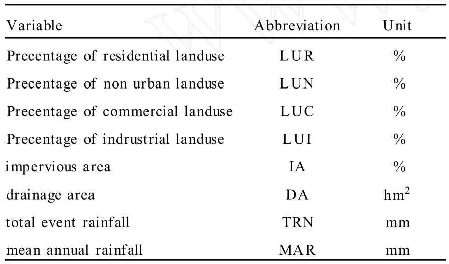
Table1 Independent variables
The data was preprocessed prior to model construction.Catchments with drainage areas greater than3 000hm2,proportions of agricultural landuse greater than50%,proportions of industrial landuse greater than50%,population densities greater than130people/hm2or with detentionbasins upstream of the sampling point were removed.A base ten logarithmic transformation was then applied to both the dependent variable and independent variables.If the variable had values equal or less than zero,aconstant was added to remap the data into a suitable domain prior to logarithmic transformation.Numerous studies indicate that water quality and other environmental variables follow lognormal distributions.Logarithmic transformation of the data ensured that large, potentially outlying values did not bias the optimisation of calibration coefficients in the models[3]. The other advantage of the logarithmic transformation was that it enabled the construction of nonlinear,nonadditive regression models using a simple multilinear regression procedure.
Error measure selection can influence the relative judgement of model performance.The standard error of estimate and average absolute percentage error do not place considerable emphasis on the large outlying values,and allow the direct comparison between models constructed using load or concentration as the dependent variable.The standard error of estimate(SEE)is a pseudo percentage error calculated from the mean square error in log(base10)units[3]:

The standard error of estimate places greater emphasis on the under prediction of large values than the average absolute percentage error (AAPE).Both the standard error of estimate and average absolute percentage error were used to compare predictions from the constructed models.
Regression models were initially constructed on a754data point set.Significant independent variables were identified using a stepwise multilinear regression analysis of the logarithmically transformed data.If the p-value of the variable was greater than0.05,the variable was entered into the model.Variables already in the model were removed if their pvalue increased above0.1.Regression models were created using total p hosp horus load and concentration as the dependent variable.O nce a series of regression models had been developed(ranging f rom a simple one variable model to more complicated multivariable models) the standard error ofestimate and average absolute percentage error were calculated. The dependent variable p roducing the minimum error was analysed in more detail.Since multiple storm events were monitored at all catchments in the data set,the majority ofindependentvariables did not satisfy the assumption of data independence.All analysed independent variables apart f rom total storm rainfall had constant values for a given catchment.This reduced the effective size of the data set,resulting in an underestimation of the p-value and the potential incorporation of spurious variables into the model.To overcome the problem, a cross validation approach was adopted.Ten disjoint data sets containing approximately10 %of the data were created.Ten analyses were undertaken,with a different set being used for validation purposes each time.The remainder of the data(90 %)was used for model calibration.Inputs were sequentially entered into the models based upon the order of entry of inputs into the stepwise regression that used all data for calibration.The average absolute percentage error and standard error of estimate were calculated for each validation set and then averaged.Variables leading to an increase in both error measures were deemed to be insignificant and removed from the model.
A second regression analysis was undertaken on a regional subset of the data.Catchments with mean annual rainfalls between500 and1 000mm were separated from the total data set,in accordance with the study by Driver and Tasker[3].These variables were analysed along with the variables found significant in the first regression analysis of the larger data set.The variables were entered into the regression model in order of their anticipated significance.A holdout method using10%of the data for validation was used to verify the significance of the independent variables.Variables not yielding improvements in the average absolute percentage error and standard error of estimate were deemed to be insignificant and removed from the model.
Feedforward,backpropagation neural networks were optimised using the normalised cummulative delta rule learning algorithm.The equation for the update of network weights is as follows:
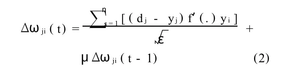
WhereΔwji=weight update between nodes i and j at time t,η=learning rate,dj=the actual output value,yj=the predicted output value,f′(.)=the derivative of the transfer function with respect to its input,ε=epoch size,μ=momentum and s=the training sample presented to the network.An epoch equal to the training set size was used to promote fast generalisation of the data.The logarithmically transformed data was scaled within the bounds of the hyperbolic tangent transer function.The input variables were scaled between -1and1,and the output variable between -0.8and0.8to encourage extrapolation.Only one hidden layer was used,due to the limited amount of data available.The learning rate for the weights connecting the input layer to the hidden layer and the hidden layer to the output layer were assumed to be0.04and0.02respectively.Momentum was assumed to be 0.01.Cross validation was used to determine when to cease network training.The data was separated into ten disjoint sets,equivalent to those defined during the regression analysis. Ten ANN models were created,using a different10%of the data as a test set each time. For each of the ten test sets,the mean square error was calculated for each weight update. An average of the mean square errors for the ten test sets was calculated for each weight update.The numberofweightupdates corresponding to the minimum average test set error was defined as the stopping point.ANN models were constructed using the dependent and independent variables found significant in the regression analysis.The effect of the number hidden nodes,learning rates and momentum on model was accuracy was also analysed.
2 Results and Discussion
The results from models constructed using stepwise regression are presented in Table2. Load models had errors more than50 %larger than the concentration models.Therefore concentration was used as the dependent variable during subsequentanalyses.Stepwise regressionswere then constructed using the965data point set.Table3compares the results from the regression analysis using100%of the data for calibration, and the regression analysis using90%of the data for calibration.The errors for the cross validation analysis using90 %of the data for calibration correspond to prediction errors,whereas the errors from the analysis using all the data for calibration were calibration errors.When cross validation was applied,only mean annual rainfall and the percentage of residential landuse lead to improvements in both the standard error of estimate and absolute average percentage error.Therefore,only these two variables were deemed to be significant on the965data point set.
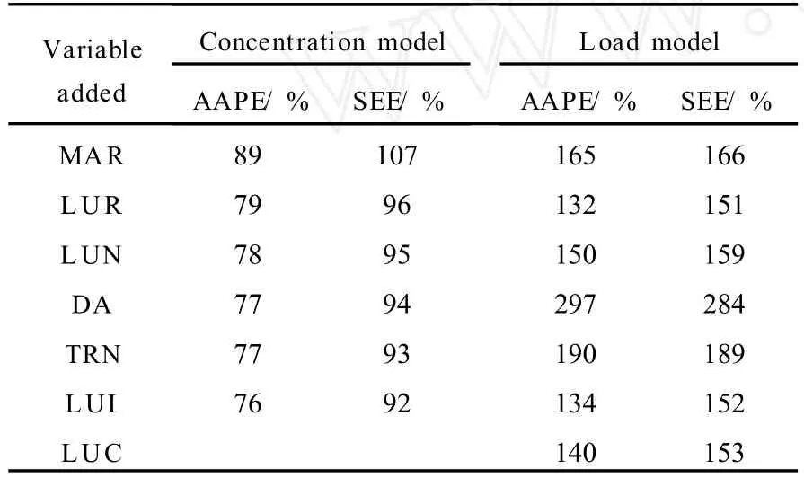
Table2 Comparison between concentration and load stepwise regression models developed on a754data point set
Regression equations were then developed on the regional subset(374data points).Results from the analysis of the larger data set justified the use of total phosphorus concentration as the dependent variable.The variables found to be significant in the study by Driver and Tasker[3]were total storm rainfall,total contributing drainage area, impervious area and maximum24-hour precipitation intensity that has a2-year recurrence interval.These variables were combined with mean annual rainfall and the percentage of residential landuse.The anticipated significance of each variable combined with information extracted from a stepwise regression determined the order of variable entry into the final regression model.The results from the analyses using100%and90%of the data for calibration are presented in Table 4. When the cross validation was applied,it was found that drainage area was the only variable that did not improve either the average absolute percentage error or standard error of estimate. Therefore,drainage area was removed from the model.Impervious area and total event rainfall only improved one error measure.However,when impervious area and total event rainfall were added together,both error measures reduced.Total event rainfall was also the only available variable in the data set capable ofdescribing storm to storm variability at a site.Therefore,total event rainfall and impervious area were left in the model.
Artificial neural networks were developed to predict total phosphorus concentration.Two independent variables were not considered to be sufficient to construct ANN models on the965data point set.Therefore,ANN models were only constructed on the regional dataset using inputs found to be significant in the regional regression analysis.Using trial and error,the optimum number of hidden nodes was found to be10.The choice of learning ratesand momentum typically determined the speed of the network convergence as well as the size of the error oscillations near the local minimum.Overall,the choice of the number of hidden nodes,learning rates and momentum had an insignificant effect upon accuracy.
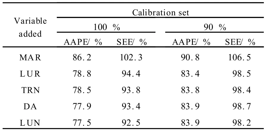
Table3 The effect of input addition on model error for regression models developed on the965data point set using total phosphorus concentration as the dependent variable

Table4 The effect of input addition on model error for regression models developed on the regional subset using total phosphorus concentration as the dependent variable
Regression and ANN models were compared on the regional data set.The results presented in Table5suggest that regression and ANN models constructed on the regional dataset had very similar accuracies.The regression model constructed using regional data was more accurate than the one constructed using all the available data.The lack of significant inputs restricted the ability of the regression modelto replicate relationships within the larger dataset,thereby reducing the accuracy of these model.
Data limitations in the current study were exacerbated by violations of data independence for the bulk of variables.Instead of analysing a large dataset equal to the number of storm events,a smaller subset equal to the number of catchments was effectively analysed.The effective size of the data set was approximately an order of magnitude smaller than the actual data set size.This made the modelled relationships tenuous and thereby decreased the likelihood of ANN and regression models to accurately predict water quality at unmonitored sites.Inaccurate predictions are inevitable without the inclusion of a significant descriptor of storm to storm variability.Total event rainfall was not significant enough to be able to define such variability.
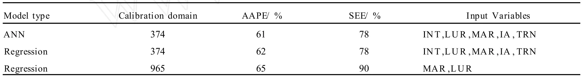
Table5 Prediction results from concentration models compared on the regional Subset
3 Conclusions
It was found that models with concentration as the dependent variable were more accurate than those with load.This was an important finding considering that the majority of current computer simulation models require estimates ofconcentration rather than load.When load was the dependent variable,the regression models were forced to simulate the known relation-ship existing between load and runoff volume,leading to an unnecessary increase in the complexity of the models.However,if the volume of runoff is not accurately known,load models might provide better estimates of the total load than the concentration models.
Violation of the assumption of data independence affected the construction of regression models. Spurious variables were entered into the model when p-values were used as the main criterion for input entry.To overcome the problem,a cross validation approach was applied to determine when to cease input addition.Regression models constructed using the total data sets were less accurate than those constructed on the regional subset of data. The reduced data complexity combined with the use of additional variables contributed to the increased accuracy of regression models constructed on the regional subset.
Compared to ANN models,regression models were faster to construct and apply,were more transparent and produced more parsimonious models.The choice of learning rates,momentum and number of hidden nodes did not significantly affect the accuracy of the ANN models.The extent of data over fitting was also greater for ANN models,due to a reliance upon the test set for the determination of optimum number of weight updates.There were no significant variables capable of describing storm to storm variability present in the dataset.The only variable capable of describing such variation was total event rainfall.However,it was found to be insignificant on the larger data set.Therefore the effective size of the available data set was considered to be too small to successfully apply ANN.
Acknowledgements
The authors would like to express their gratitude to Pam Davy for her insights and general assistance during the course of the research.
[1] Barks C S.Ajustment of Regional Regression Equations for Urban Storm-runoff Quality Using At-stie Data [J].Transportation Research Record,1996(1523):141 -146.
[2] Brezonik P L,Stadelmann T H.Analysis and Predictive Models of Stormwater Runoff Volumes,Loads,and Pollutant Concentrations from Watersheds in the Twin Cities Metropolitan Area,Minnesota,USA[J].Water Research,2002,36(7):1743-1757.
[3] Driver N,TaskerG.Techniques for Estimation of Storm-runoff Loads,Volumes,and Selected Consituent Concentrations in Urban Watersheds in the United States[R].Washington:United StatesGovernment Printing Office:1990.
[4] Sliva L,Williams D D.Buffer Zone Versus Whole Catchment Approaches to Studying Land Use Impact on River Water Quality[J].Water Research,2001,35 (14):3462-3472.
[5] Smullen J T,Shallcross A L,Cave K A.Updating the U.S.Nationwide Urban Runoff Quality Data Base[J]. Water Science and Technology,1999,39(12):9-16.
[6] Lek S,Guiresse M,Giraudel J.Predicting Stream Nitrogen Concentration from Watershed Features Using NeuralNetworks[J].Water Research, 1999,33(16):3469-3478.
[7] Maier H R,Dandy G C.The Effect of Internal Parameters and Geometry on the Performance of Back-propagation Neural Networks:and Empirical Study[J].Environmental Modelling and Software, 1998,13(2):193-209.
[8] Maier H R,Dandy G C.Neural Networks for the Prediction and Forecasting ofWaterResources Variables:a Review of Modeling Issues and Applications[J].Environmental Modelling and Software,2000,15(1):101-124.
[9] Cahaba/Warrior Student Chapter of the American Water Resources Association(University of Alabama).NU RP data[EB/OL].1998-03-05. [2009-10-15]http://www.eng.ua.edu/~awra/download.htm.